|
|
| (448 intermediate revisions by the same user not shown) |
| Line 1: |
Line 1: |
| − | ==Sediment Porewater Dialysis Passive Samplers for Inorganics (Peepers)== | + | ==Estimating PCE/TCE Abiotic First-Order Reductive Dechlorination Rate Constants in Clayey Soils Under Anoxic Conditions== |
| − | Sediment porewater dialysis passive samplers, also known as “peepers,” are sampling devices that allow the measurement of dissolved inorganic ions in the porewater of a saturated sediment. Peepers function by allowing freely-dissolved ions in sediment porewater to diffuse across a micro-porous membrane towards water contained in an isolated compartment that has been inserted into sediment. Once retrieved after a deployment period, the resulting sample obtained can provide concentrations of freely-dissolved inorganic constituents in sediment, which provides measurements that can be used for understanding contaminant fate and risk. Peepers can also be used in the same manner in surface water, although this article is focused on the use of peepers in sediment.
| + | The U.S. Department of Defense (DoD) faces many challenges in restoring aquifers at contaminated sites, often due to back-diffusion of tetrachloroethene (PCE) and trichloroethene (TCE) from low-permeability clay zones. The uptake, storage, and subsequent long-term release of these dissolved contaminants from clays are key processes in understanding the longevity, intensity, and risks associated with many persistent chlorinated ethene groundwater plumes. Although naturally occurring abiotic and biotic dechlorination processes in clays may reduce stored contaminant mass and significantly aid natural attenuation, no standardized field method currently exists to verify or quantify these reactions. It is critical to remediation design efforts to demonstrate and validate a cost-effective in situ approach for assessing these dechlorination processes using first-order rate constants. An approach was developed and applied across eight DoD sites to support Remedial Project Managers (RPMs) and regulators in evaluating natural attenuation potential in clay-rich environments. |
| − | | |
| | <div style="float:right;margin:0 0 2em 2em;">__TOC__</div> | | <div style="float:right;margin:0 0 2em 2em;">__TOC__</div> |
| | | | |
| | '''Related Article(s):''' | | '''Related Article(s):''' |
| | | | |
| − | *[[Contaminated Sediments - Introduction]] | + | *[[Monitored Natural Attenuation (MNA)]] |
| − | *[[Contaminated Sediment Risk Assessment]] | + | *[[Monitored Natural Attenuation (MNA) of Chlorinated Solvents]] |
| − | *[[In Situ Treatment of Contaminated Sediments with Activated Carbon]]
| + | *[[Monitored Natural Attenuation - Transitioning from Active Remedies]] |
| − | *[[Passive Sampling of Munitions Constituents]] | + | *[[Matrix Diffusion]] |
| − | *[[Sediment Capping]] | + | *[[REMChlor - MD]] |
| − | *[[Mercury in Sediments]] | |
| − | *[[Passive Sampling of Sediments]]
| |
| − | | |
| − | | |
| − | '''Contributor(s):'''
| |
| | | | |
| − | *Florent Risacher, M.Sc.
| + | '''Contributors:''' Dani Tran, Dr. Charles Schaefer, Dr. Charles Werth |
| − | *Jason Conder, Ph.D.
| |
| | | | |
| − | '''Key Resource(s):''' | + | '''Key Resource:''' |
| − | | + | *Schaefer, C.E, Tran, D., Nguyen, D., Latta, D.E., Werth, C.J., 2025. Evaluating Mineral and In Situ Indicators of Abiotic Dechlorination in Clayey Soils<ref name="SchaeferEtAl2025"/> |
| − | *A review of peeper passive sampling approaches to measure the availability of inorganics in sediment porewater<ref>Risacher, F.F., Schneider, H., Drygiannaki, I., Conder, J., Pautler, B.G., and Jackson, A.W., 2023. A Review of Peeper Passive Sampling Approaches to Measure the Availability of Inorganics in Sediment Porewater. Environmental Pollution, 328, Article 121581. [https://doi.org/10.1016/j.envpol.2023.121581 doi: 10.1016/j.envpol.2023.121581] [[Media: RisacherEtAl2023a.pdf | Open Access Manuscript]]</ref> | |
| − | | |
| − | *Best Practices User’s Guide: Standardizing Sediment Porewater Passive Samplers for Inorganic Constituents of Concern<ref name="RisacherEtAl2023">Risacher, F.F., Nichols, E., Schneider, H., Lawrence, M., Conder, J., Sweett, A., Pautler, B.G., Jackson, W.A., Rosen, G., 2023b. Best Practices User’s Guide: Standardizing Sediment Porewater Passive Samplers for Inorganic Constituents of Concern, ESTCP ER20-5261. [https://serdp-estcp.mil/projects/details/db871313-fbc0-4432-b536-40c64af3627f Project Website] [[Media: ER20-5261BPUG.pdf | Report.pdf]]</ref>
| |
| − | | |
| − | *[https://serdp-estcp.mil/projects/details/db871313-fbc0-4432-b536-40c64af3627f/er20-5261-project-overview Standardizing Sediment Porewater Passive Samplers for Inorganic Constituents of Concern, ESTCP Project ER20-5261]
| |
| | | | |
| | ==Introduction== | | ==Introduction== |
| − | Biologically available inorganic constituents associated with sediment toxicity can be quantified by measuring the freely-dissolved fraction of contaminants in the porewater<ref>Conder, J.M., Fuchsman, P.C., Grover, M.M., Magar, V.S., Henning, M.H., 2015. Critical review of mercury SQVs for the protection of benthic invertebrates. Environmental Toxicology and Chemistry, 34(1), pp. 6-21. [https://doi.org/10.1002/etc.2769 doi: 10.1002/etc.2769] [[Media: ConderEtAl2015.pdf | Open Access Article]]</ref><ref name="ClevelandEtAl2017">Cleveland, D., Brumbaugh, W.G., MacDonald, D.D., 2017. A comparison of four porewater sampling methods for metal mixtures and dissolved organic carbon and the implications for sediment toxicity evaluations. Environmental Toxicology and Chemistry, 36(11), pp. 2906-2915. [https://doi.org/10.1002/etc.3884 doi: 10.1002/etc.3884]</ref>. Classical sediment porewater analysis usually consists of collecting large volumes of bulk sediments which are then mechanically squeezed or centrifuged to produce a supernatant, or suction of porewater from intact sediment, followed by filtration and collection<ref name="GruzalskiEtAl2016">Gruzalski, J.G., Markwiese, J.T., Carriker, N.E., Rogers, W.J., Vitale, R.J., Thal, D.I., 2016. Pore Water Collection, Analysis and Evolution: The Need for Standardization. In: Reviews of Environmental Contamination and Toxicology, Vol. 237, pp. 37–51. Springer. [https://doi.org/10.1007/978-3-319-23573-8_2 doi: 10.1007/978-3-319-23573-8_2]</ref>. The extraction and measurement processes present challenges due to the heterogeneity of sediments, physical disturbance, high reactivity of some complexes, and interaction between the solid and dissolved phases, which can impact the measured concentration of dissolved inorganics<ref>Peijnenburg, W.J.G.M., Teasdale, P.R., Reible, D., Mondon, J., Bennett, W.W., Campbell, P.G.C., 2014. Passive Sampling Methods for Contaminated Sediments: State of the Science for Metals. Integrated Environmental Assessment and Management, 10(2), pp. 179–196. [https://doi.org/10.1002/ieam.1502 doi: 10.1002/ieam.1502] [[Media: PeijnenburgEtAl2014.pdf | Open Access Article]]</ref>. For example, sampling disturbance can affect redox conditions<ref name="TeasdaleEtAl1995">Teasdale, P.R., Batley, G.E., Apte, S.C., Webster, I.T., 1995. Pore water sampling with sediment peepers. Trends in Analytical Chemistry, 14(6), pp. 250–256. [https://doi.org/10.1016/0165-9936(95)91617-2 doi: 10.1016/0165-9936(95)91617-2]</ref><ref>Schroeder, H., Duester, L., Fabricius, A.L., Ecker, D., Breitung, V., Ternes, T.A., 2020. Sediment water (interface) mobility of metal(loid)s and nutrients under undisturbed conditions and during resuspension. Journal of Hazardous Materials, 394, Article 122543. [https://doi.org/10.1016/j.jhazmat.2020.122543 doi: 10.1016/j.jhazmat.2020.122543] [[Media: SchroederEtAl2020.pdf | Open Access Article]]</ref>, which can lead to under or over representation of inorganic chemical concentrations relative to the true dissolved phase concentration in the sediment porewater<ref>Wise, D.E., 2009. Sampling techniques for sediment pore water in evaluation of reactive capping efficacy. Master of Science Thesis. University of New Hampshire Scholars’ Repository. 178 pages. [https://scholars.unh.edu/thesis/502 Website] [[Media: Wise2009.pdf | Report.pdf]]</ref><ref name="GruzalskiEtAl2016"/>.
| + | Cost-effective methods are needed to verify the occurrence of natural dechlorination processes and quantify their dechlorination rates in clays under ambient in situ conditions in order to reliably predict their long-term influence on plume longevity and mass discharge. However, accurately determining these rates is challenging due to slow reaction kinetics, the transient nature of transformation products, and the interplay of biotic and abiotic mechanisms within the clay matrix or at clay-sand interfaces. Tools capable of quantifying these reactions and assessing their role in mitigating plume persistence would be a significant aid for long-term site management. |
| − | | |
| − | To address the complications with mechanical porewater sampling, passive sampling approaches for inorganics have been developed to provide a method that has a low impact on the surrounding geochemistry of sediments and sediment porewater, thus enabling more precise measurements of inorganics<ref name="ClevelandEtAl2017"/>. Sediment porewater dialysis passive samplers, also known as “peepers,” were developed more than 45 years ago<ref name="Hesslein1976">Hesslein, R.H., 1976. An in situ sampler for close interval pore water studies. Limnology and Oceanography, 21(6), pp. 912-914. [https://doi.org/10.4319/lo.1976.21.6.0912 doi: 10.4319/lo.1976.21.6.0912] [[Media: Hesslein1976.pdf | Open Access Article]]</ref> and refinements to the method such as the use of reverse tracers have been made, improving the acceptance of the technology as decision-making tool.
| |
| − | | |
| − | ==Peeper Designs==
| |
| − | [[File:RisacherFig1.png|thumb|300px|Figure 1. Conceptual illustration of peeper construction showing (top, left to right) the peeper cap (optional), peeper membrane and peeper chamber, and (bottom) an assembled peeper containing peeper water]]
| |
| − | [[File:RisacherFig2.png | thumb |400px| Figure 2. Example of Hesslein<ref name="Hesslein1976"/> general peeper design (42 peeper chambers), from [https://www.usgs.gov/media/images/peeper-samplers USGS]]]
| |
| − | [[File:RisacherFig3.png | thumb |400px| Figure 3. Peeper deployment structure to allow the measurement of metal availability in different sediment layers using five single-chamber peepers (Photo: Geosyntec Consultants)]]
| |
| − | Peepers (Figure 1) are inert containers with a small volume (typically 1-100 mL) of purified water (“peeper water”) capped with a semi-permeable membrane. Peepers can be manufactured in a wide variety of formats (Figure 2, Figure 3) and deployed in in various ways.
| |
| − | | |
| − | Two designs are commonly used for peepers. Frequently, the designs are close adaptations of the original multi-chamber Hesslein design<ref name="Hesslein1976"/> (Figure 2), which consists of an acrylic sampler body with multiple sample chambers machined into it. Peeper water inside the chambers is separated from the outside environment by a semi-permeable membrane, which is held in place by a top plate fixed to the sampler body using bolts or screws. An alternative design consists of single-chamber peepers constructed using a single sample vial with a membrane secured over the mouth of the vial, as shown in Figure 3, and applied in Teasdale ''et al.''<ref name="TeasdaleEtAl1995"/>, Serbst ''et al.''<ref>Serbst, J.R., Burgess, R.M., Kuhn, A., Edwards, P.A., Cantwell, M.G., Pelletier, M.C., Berry, W.J., 2003. Precision of dialysis (peeper) sampling of cadmium in marine sediment interstitial water. Archives of Environmental Contamination and Toxicology, 45(3), pp. 297–305. [https://doi.org/10.1007/s00244-003-0114-5 doi: 10.1007/s00244-003-0114-5]</ref>, Thomas and Arthur<ref name="ThomasArthur2010">Thomas, B., Arthur, M.A., 2010. Correcting porewater concentration measurements from peepers: Application of a reverse tracer. Limnology and Oceanography: Methods, 8(8), pp. 403–413. [https://doi.org/10.4319/lom.2010.8.403 doi: 10.4319/lom.2010.8.403] [[Media: ThomasArthur2010.pdf | Open Access Article]]</ref>, Passeport ''et al.''<ref>Passeport, E., Landis, R., Lacrampe-Couloume, G., Lutz, E.J., Erin Mack, E., West, K., Morgan, S., Lollar, B.S., 2016. Sediment Monitored Natural Recovery Evidenced by Compound Specific Isotope Analysis and High-Resolution Pore Water Sampling. Environmental Science and Technology, 50(22), pp. 12197–12204. [https://doi.org/10.1021/acs.est.6b02961 doi: 10.1021/acs.est.6b02961]</ref>, and Risacher ''et al.''<ref name="RisacherEtAl2023"/>. The vial is filled with deionized water, and the membrane is held in place using the vial cap or an o-ring. Individual vials are either directly inserted into sediment or are incorporated into a support structure to allow multiple single-chamber peepers to be deployed at once over a given depth profile (Figure 3).
| |
| − | | |
| − | ==Peepers Preparation, Deployment and Retrieval==
| |
| − | [[File:RisacherFig4.png | thumb |400px| Figure 4: Conceptual illustration of peeper passive sampling in a sediment matrix, showing peeper immediately after deployment (top) and after equilibration between the porewater and peeper chamber water (bottom)]]
| |
| − | Peepers are often prepared in laboratories but are also commercially available in a variety of designs from several suppliers. Peepers are prepared by first cleaning all materials to remove even trace levels of metals before assembly. The water contained inside the peeper is sometimes deoxygenated, and in some cases the peeper is maintained in a deoxygenated atmosphere until deployment<ref>Carignan, R., St‐Pierre, S., Gachter, R., 1994. Use of diffusion samplers in oligotrophic lake sediments: Effects of free oxygen in sampler material. Limnology and Oceanography, 39(2), pp. 468-474. [https://doi.org/10.4319/lo.1994.39.2.0468 doi: 10.4319/lo.1994.39.2.0468] [[Media: CarignanEtAl1994.pdf | Open Access Article]]</ref>. However, recent studies<ref name="RisacherEtAl2023"/> have shown that deoxygenation prior to deployment does not significantly impact sampling results due to oxygen rapidly diffusing out of the peeper during deployment. Once assembled, peepers are usually shipped in a protective bag inside a hard-case cooler for protection.
| |
| − | | |
| − | Peepers are deployed by insertion into sediment for a period of a few days to a few weeks. Insertion into the sediment can be achieved by wading to the location when the water depth is shallow, by using push poles for deeper deployments<ref name="RisacherEtAl2023"/>, or by professional divers for the deepest sites. If divers are used, an appropriate boat or ship will be required to accommodate the diver and their equipment. Whichever method is used, peepers should be attached to an anchor or a small buoy to facilitate retrieval at the end of the deployment period.
| |
| − | | |
| − | During deployment, passive sampling is achieved via diffusion, as the enclosed volume of peeper water equilibrates with the surrounding sediment porewater via transport of inorganics through the peeper’s semi-permeable membrane (Figure 4). It is assumed that the peeper insertion does not greatly alter geochemical conditions that affect freely-dissolved inorganics. Additionally, it is assumed that the peeper water equilibrates with freely-dissolved inorganics in sediment in such a way that the concentration of inorganics in the peeper water would be equal to that of the concentration of inorganics in the sediment porewater.
| |
| − | | |
| − | After retrieval, the peepers are brought to the surface and usually preserved until they can be processed. This can be achieved by storing the peepers inside a sealable, airtight bag with either inert gas or oxygen absorbing packets<ref name="RisacherEtAl2023"/>. The peeper water can then be processed by quickly pipetting it into an appropriate sample bottle which usually contains a preservative (e.g., nitric acid for metals). This step is generally conducted in the field. Samples are stored on ice to maintain a temperature of less than 4°C and shipped to an analytical laboratory. The samples are then analyzed for inorganics by standard methods (i.e., USEPA SW-846). The results obtained from the analytical laboratory are then used directly or assessed using the equations below if a reverse tracer is used because deployment time is insufficient for all analytes to reach equilibrium.
| |
| | | | |
| − | ==Equilibrium Determination (Tracers)==
| + | For reductive abiotic dechlorination under anoxic conditions, a 1% hydrochloric acid (HCl) extraction of a sample of native clay coupled with X-ray diffraction (XRD) data can be used as a screening level tool to estimate reductive dechlorination rate constants. These rate constants can be inserted into fate and transport models such as [[REMChlor - MD]]<ref>Falta, R., and Wang, W., 2017. A semi-analytical method for simulating matrix diffusion in numerical transport models. Journal of Contaminant Hydrology, 197, pp. 39-49. [https://doi.org/10.1016/j.jconhyd.2016.12.007 doi: 10.1016/j.jconhyd.2016.12.007] [[Media: FaltaWang2017.pdf | Open Access Manuscript]]</ref><ref>Kulkarni, P.R., Adamson, D.T., Popovic, J., Newell, C.J., 2022. Modeling a well-charactized perfluorooctane sulfate (PFOS) source and plume using the REMChlor-MD model to account for matrix diffusion. Journal of Contaminant Hydrology, 247, Article 103986. [https://doi.org/10.1016/j.jconhyd.2022.103986 doi: 10.1016/j.jconhyd.2022.103986] [[Media: KulkarniEtAl2022.pdf | Open Access Manuscript]]</ref> to quantify abiotic dechlorination impacts within clay aquitards on chlorinated solvent plumes. Thus, determination of the abiotic reductive dechlorination rate constant for a particular clayey soil can be readily utilized to provide a more accurate assessment of aquifer cleanup timeframes for groundwater plumes that are being sustained by contaminant back-diffusion. |
| − | The equilibration period of peepers can last several weeks and depends on deployment conditions, analyte of interest, and peeper design. In many cases, it is advantageous to use pre-equilibrium methods that can use measurements in peepers deployed for shorter periods to predict concentrations at equilibrium<ref name="USEPA2017">USEPA, 2017. Laboratory, Field, and Analytical Procedures for Using Passive Sampling in the Evaluation of Contaminated Sediments: User’s Manual. EPA/600/R-16/357. [[Media: EPA_600_R-16_357.pdf | Report.pdf]]</ref>.
| |
| | | | |
| − | Although the equilibrium concentration of an analyte in sediment can be evaluated by examining analyte results for peepers deployed for several different amounts of time (i.e., a time series), this is impractical for typical field investigations because it would require several mobilizations to the site to retrieve samplers. Alternately, reverse tracers (referred to as a performance reference compound when used with organic compound passive sampling) can be used to evaluate the percentage of equilibrium reached by a passive sampler.
| + | ==Recommended Approach== |
| | + | [[File: TranFig1.png | thumb | 500 px | Figure 1: First-order rate constants for abiotic reductive dechlorination of TCE under anaerobic conditions. Circles are data from Schaefer ''et al.'', 2021<ref>Schaefer, C.E., Ho, P., Berns, E., Werth, C., 2021. Abiotic dechlorination in the presence of ferrous minerals. Journal of Contaminant Hydrology, 241, 103839. [https://doi.org/10.1016/j.jconhyd.2021.103839 doi: 10.1016/j.jconhyd.2021.103839] [[Media: SchaeferEtAl2021.pdf | Open Access Manuscript]]</ref>, filled squares from Schaefer ''et al.'', 2018<ref name="SchaeferEtAl2018"/>, and Schaefer ''et al.'', 2017<ref>Schaefer, C.E., Ho., Gurr, C., Berns, E., Werth, C., 2017. Abiotic dechlorination of chlorinated ethenes in natural clayey soils: impacts of mineralogy and temperature. Journal of Contaminant Hydrology, 206, pp. 10-17. [https://doi.org/10.1016/j.jconhyd.2017.09.007 doi: 10.1016/j.jconhyd.2017.09.007] [[Media: SchaeferEtAl2017.pdf | Open Access Manuscript]]</ref>, and open squares from Schaefer ''et al.'', 2025<ref name="SchaeferEtAl2025"/>. ]] |
| | + | [[File: TranFig2.png | thumb | 600 px | Figure 2: Flowchart diagram of field screening procedures]] |
| | + | The recommended approach builds upon the methodology and findings of a recent study<ref name="SchaeferEtAl2025">Schaefer, C.E., Tran, D., Nguyen, D., Latta, D.E., Werth, C.J., 2025. Evaluating Mineral and In Situ Indicators of Abiotic Dechlorination in Clayey Soils. Groundwater Monitoring and Remediation, 45(2), pp. 31-39. [https://doi.org/10.1111/gwmr.12709 doi: 10.1111/gwmr.12709]</ref>, emphasizing field-based and analytical techniques to quantify abiotic first-order reductive dechlorination rate constants for PCE and TCE in clayey soils under anoxic conditions. Key components of this evaluation are listed below: |
| | + | #<u>Zone Identification:</u> The focus of the investigation should be to delineate clayey zones adjacent to hydraulically conductive zones. |
| | + | #<u>Ferrous Mineral Quantification:</u> Assess ferrous mineral context in clay via 1% HCl extraction at ambient temperature over a 10-minute interval. |
| | + | #<u>Mineralogical Characterization:</u> Conduct XRD analysis with the specific intent of identifying the presence of pyrite and biotite. |
| | + | #<u>Reduced Gas Analysis:</u> Measurement of reduced gases such as acetylene, ethene, and ethane concentrations in clay samples. Gas-tight sampling devices (e.g., En Core® soil samplers by En Novative Technologies, Inc.) should be used to ensure sample integrity during collection and transport. |
| | | | |
| − | Thomas and Arthur<ref name="ThomasArthur2010"/> studied the use of a reverse tracer to estimate percent equilibrium in lab experiments and a field application. They concluded that bromide can be used to estimate concentrations in porewater using measurements obtained before equilibrium is reached. Further studies were also conducted by Risacher ''et al.''<ref name="RisacherEtAl2023"/> showed that lithium can also be used as a tracer for brackish and saline environments. Both studies included a mathematical model for estimating concentrations of ions in external media (''C<small><sub>0</sub></small>'') based on measured concentrations in the peeper chamber (''C<small><sub>p,t</sub></small>''), the elimination rate of the target analyte (''K'') and the deployment time (''t''):
| + | Clay samples should be collected within a few centimeters of the high-permeability interface, with optional additional sampling further inward. For mineralogical analysis, a defined interval may be collected and subsequently subsampled. To preserve sample integrity, exposure to air should be minimized during collection, transport, and handling. Homogenization should occur within an anaerobic chamber, and if subsamples are required for external analysis, they must be shipped in gas-tight, anaerobic containers. |
| − | </br>
| |
| − | {|
| |
| − | | || '''Equation 1:'''
| |
| − | | [[File: Equation1r.png]]
| |
| − | |-
| |
| − | | Where: || ||
| |
| − | |-
| |
| − | | || ''C<small><sub>0</sub></small>''|| is the freely dissolved concentration of the analyte in the sediment (mg/L or μg/L), sometimes referred to as ''C<small><sub>free</sub></small>
| |
| − | |-
| |
| − | | || ''C<small><sub>p,t</sub></small>'' || is the measured concentration of the analyte in the peeper at time of retrieval (mg/L or μg/L)
| |
| − | |-
| |
| − | | || ''K'' || is the elimination rate of the target analyte
| |
| − | |-
| |
| − | | || ''t'' || is the deployment time (days)
| |
| − | |}
| |
| | | | |
| − | The elimination rate of the target analyte (''K'') is calculated using Equation 2:
| + | Estimation of the abiotic reductive first-order rate constant for PCE and TCE is based on the “reactive” ferrous content in the clay. Reactive ferrous content (Fe(II)<sub>r</sub>) is estimated as shown in Equation 1: |
| − | </br>
| |
| − | {|
| |
| − | | || '''Equation 2:'''
| |
| − | | [[File: Equation2r.png]]
| |
| − | |-
| |
| − | | Where: || ||
| |
| − | |-
| |
| − | | || ''K''|| is the elimination rate of the target analyte
| |
| − | |-
| |
| − | | || ''K<small><sub>tracer</sub></small>'' || is the elimination rate of the tracer
| |
| − | |-
| |
| − | | || ''D'' || is the free water diffusivity of the analyte (cm<sup>2</sup>/s)
| |
| − | |-
| |
| − | | || ''D<small><sub>tracer</sub></small>'' || is the free water diffusivity of the tracer (cm<sup>2</sup>/s)
| |
| − | |}
| |
| | | | |
| − | The elimination rate of the tracer (''K<small><sub>tracer</sub></small>'') is calculated using Equation 3:
| + | ::'''Equation 1:''' <big>''Fe(II)<sub><small>r</small></sub> = DA + XRD<sub><small>pyr</small></sub> - XRD<sub><small>biotite</small></sub>''</big> |
| − | </br>
| |
| − | {|
| |
| − | | || '''Equation 3:'''
| |
| − | | [[File: Equation3r2.png]]
| |
| − | |-
| |
| − | | Where: || ||
| |
| − | |-
| |
| − | | || ''K<small><sub>tracer</sub></small>'' || is the elimination rate of the tracer
| |
| − | |-
| |
| − | | || ''C<small><sub>tracer,i</sub></small>''|| is the measured initial concentration of the tracer in the peeper prior to deployment (mg/L or μg/L)
| |
| − | |-
| |
| − | | || ''C<small><sub>tracer,t</sub></small>'' || is the measured final concentration of the tracer in the peeper at time of retrieval (mg/L or μg/L)
| |
| − | |-
| |
| − | | || ''t'' || is the deployment time (days)
| |
| − | |}
| |
| | | | |
| − | Using this set of equations allows the calculation of the porewater concentration of the analyte at equilibrium. A template for these calculations can be found in the appendix of Risacher ''et al.''<ref name="RisacherEtAl2023"/>
| + | where ''DA'' is the ferrous content from the dilute acid (1% HCl) extraction, ''XRD<sub><small>pyr</small></sub>'' is the pyrite content from XRD analysis, and ''XRD<sub><small>biotite</small></sub>'' is the biotite content from XRD analysis<ref name="SchaeferEtAl2025"/>. |
| | | | |
| − | ==Using Peeper Data at a Sediment Site==
| + | Abiotic dechlorination is unlikely to contribute to mitigating contaminant back-diffusion when reactive ferrous iron (Fe(II)<sub><small>r</small></sub>) concentrations are below 100 mg/kg (Figure 1). For Fe(II)<sub><small>r</small></sub> above 100 mg/kg, the first-order rate constant for PCE and TCE reductive dechlorination can be estimated using the correlation shown in Figure 1<ref name="SchaeferEtAl2018">Schaefer, C.E., Ho, P., Berns, E., Werth, C., 2018. Mechanisms for abiotic dechlorination of trichloroethene by ferrous minerals under oxic and anoxic conditions in natural sediments. Environmental Science and Technology, 52(23), pp.13747-13755. [https://doi.org/10.1021/acs.est.8b04108 doi: 10.1021/acs.est.8b04108]</ref><ref>Borden, R.C., Cha, K.Y., 2021. Evaluating the impact of back diffusion on groundwater cleanup time. Journal of Contaminant Hydrology, 243, Article 103889. [https://doi.org/10.1016/j.jconhyd.2021.103889 doi: 10.1016/j.jconhyd.2021] [[Media: BordenCha2021.pdf | Open Access Manuscript]]</ref>. The rate constant exhibits a strong positive correlation with the logarithm of reactive Fe(II) content (Pearson’s ''r'' = 0.82), with a slope of 4.7 × 10⁻⁸ L g⁻¹ d⁻¹ (log mg kg⁻¹)⁻¹. |
| − | Peeper data can be used to enable site specific decision making in a variety of ways. Some of the most common uses for peepers and peeper data are discussed below.
| |
| | | | |
| − | '''Nature and Extent:''' Multiple peepers deployed in sediment can help delineate areas of increased metal availability. Peepers are especially helpful for sites that are comprised of coarse, relatively inert materials that may not be conducive to traditional bulk sediment sampling. Because much of the inorganics present in these types of sediments may be associated with the porewater phase rather than the solid phase, peepers can provide a more representative measurement of C<small><sub>0</sub></small>. Additionally, at sites where tidal pumping or groundwater flux may be influencing the nature and extent of inorganics, peepers can provide a distinct advantage to bulk sediment sampling or other point-in-time measurements, as peepers can provide an average measurement that integrates the variability in the hydrodynamic and chemical conditions over time.
| + | Figure 2 presents a decision flowchart designed to evaluate the significance and extent of abiotic reductive dechlorination. By applying Equation 1 to the dilute acid extractable Fe(II) plus measured mineral species data from clay samples, the reactive ferrous iron content (Fe(II)<sub><small>r</small></sub>) can be quantified, enabling a streamlined assessment of the extent to which abiotic processes are contributing to the mitigation of contaminant back-diffusion. |
| | | | |
| − | '''Sources and Fate:''' A considerable advantage to using peepers is that C<small><sub>0</sub></small> results are expressed as concentration in units of mass per volume (e.g., mg/L), providing a common unit of measurement to compare across multiple media. For example, synchronous measurements of C<small><sub>0</sub></small> using peepers deployed in both surface water and sediment can elucidate the potential flux of inorganics from sediment to surface water. Paired measurements of both C<small><sub>0</sub></small> and bulk metals in sediment can also allow site specific sediment-porewater partition coefficients to be calculated. These values can be useful in understanding and predicting contaminant fate, especially in situations where the potential dissolution of metals from sediment are critical to predict, such as when sediment is dredged.
| + | If Fe(II)r is ≥ 100 mg/kg, a first-order dechlorination rate constant can be estimated and subsequently used within a contaminant fate and transport model. However, if acetylene is detected in the clay, even with Fe(II)r less than 100 mg/kg, then bench-scale testing using methods similar to those described in a recent study<ref name="SchaeferEtAl2025"/> is recommended, as such results would likely be inconsistent with those shown in Figure 1, suggesting some other mechanism might be involved, or that the system mineralogy might be more complex than anticipated. Even if Fe(II)r ≥ 100 mg/kg, confirmatory bench-scale testing may be conducted for additional verification and to refine estimation of the abiotic dechlorination rate constant. |
| | | | |
| − | '''Direct Toxicity to Aquatic Life:''' Peepers are frequently used to understand the potential direct toxicity to aquatic life, such as benthic invertebrates and fish. A C<small><sub>0</sub></small> measurement obtained from a peeper deployed in sediment (''in situ'') or surface water (''ex situ''), can be compared to toxicological benchmarks for aquatic life to understand the potential toxicity to aquatic life and to set remediation goals<ref name="USEPA2017"/>. C<small><sub>0</sub></small> measurements can also be incorporated in more sophisticated approaches, such as the Biotic Ligand Model<ref>Santore, C.R., Toll, E.J., DeForest, K.D., Croteau, K., Baldwin, A., Bergquist, B., McPeek, K., Tobiason, K., and Judd, L.N., 2022. Refining our understanding of metal bioavailability in sediments using information from porewater: Application of a multi-metal BLM as an extension of the Equilibrium Partitioning Sediment Benchmarks. Integrated Environmental Assessment and Management, 18(5), pp. 1335–1347. [https://doi.org/10.1002/ieam.4572 doi: 10.1002/ieam.4572]</ref> to understand the potential for toxicity or the need to conduct toxicological testing or ecological evaluations.
| + | ==Summary and Recommendations== |
| | + | The approach outlined above is intended to serve as a generalized guide for practitioners and site managers to cost-effectively determine the extent to which beneficial abiotic reductive dechlorination reactions are likely occurring in low permeability (e.g., clayey) zones. This approach may be contraindicated if co-contaminants are present. It is currently unclear whether other classes of potentially reactive chemicals, such as trinitrotoluene (TNT) or chlorinated ethanes, could interact competitively with PCE and TCE. |
| | | | |
| − | '''Bioaccumulation of Inorganics by Aquatic Life:''' Peepers can also be used to understand site specific relationship between C<small><sub>0</sub></small> and concentrations of inorganics in aquatic life. For example, measuring C<small><sub>0</sub></small> in sediment from which organisms are collected and analyzed can enable the estimation of a site-specific uptake factor. This C<small><sub>0</sub></small>-to-organism uptake factor (or model) can then be applied for a variety of uses, including predicting the concentration of inorganics in other organisms, or estimating a sediment C<small><sub>0</sub></small> value that would be safe for consumption by wildlife or humans. Because several decades of research have found that the correlation between C<small><sub>0</sub></small> measurements and bioavailability is usually better than the correlation between measurements of chemicals in bulk sediment and bioavailability, C<small><sub>0</sub></small>-to-organism uptake factors are likely to be more accurate than uptake factors based on bulk sediment testing.
| + | In addition, it remains unclear how other classes of compounds such as per- and polyfluoroalkyl substances (PFAS) may interact or sorb with ferrous minerals and potentially inhibit abiotic dechlorination reactions. Coupling these recommended activities with conventional site investigation tasks would provide an opportunity to perform many of the up-front screening activities with minimal additional project costs. It is important to note that the guidance proposed herein pertains to particularly low permeability media. Sites with complex or varying lithology, where the mineralogy and/or redox conditions may vary, might require evaluation of multiple samples to provide appropriate site-wide information. |
| | | | |
| − | '''Evaluating Sediment Remediation Efficacy:''' Passive sampling has been used widely to evaluate the efficacy of remedial actions such as active amendments, thin layer placements, and capping to reduce the availability of contaminants at sediment sites. A particularly powerful approach is to compare baseline (pre-remedy) C<small><sub>0</sub></small> in sediment to C<small><sub>0</sub></small> in sediment after the sediment remedy has been applied. Peepers can be used in this context for inorganics, allowing the sediment remedy’s success to be evaluated and monitored in laboratory benchtop remedy evaluations, pilot scale remedy evaluations, and full-scale remediation monitoring.
| + | <br clear="right"/> |
| | | | |
| | ==References== | | ==References== |
| Line 126: |
Line 55: |
| | | | |
| | ==See Also== | | ==See Also== |
| − | *[https://vimeo.com/809180171/c276c1873a Peeper Deployment Video] | + | *[https://serdp-estcp.mil/projects/details/a7e3f7b5-ed82-4591-adaa-6196ff33dd60 ESTCP Project ER20-5031 – In Situ Verification and Quantification of Naturally Occurring Dechlorination Rates in Clays: Demonstrating Processes that Mitigate Back-Diffusion and Plume Persistence] |
| − | *[https://vimeo.com/811073634/303edf2693 Peeper Retrieval Video]
| |
| − | *[https://vimeo.com/811328715/aea3073540 Peeper Processing Video]
| |
| − | *[https://sepub-prod-0001-124733793621-us-gov-west-1.s3.us-gov-west-1.amazonaws.com/s3fs-public/2024-09/ER20-5261%20Fact%20Sheet.pdf?VersionId=malAixSQQM3mWCRiaVaxY8wLdI0jE1PX Fact Sheet]
| |
Estimating PCE/TCE Abiotic First-Order Reductive Dechlorination Rate Constants in Clayey Soils Under Anoxic Conditions
The U.S. Department of Defense (DoD) faces many challenges in restoring aquifers at contaminated sites, often due to back-diffusion of tetrachloroethene (PCE) and trichloroethene (TCE) from low-permeability clay zones. The uptake, storage, and subsequent long-term release of these dissolved contaminants from clays are key processes in understanding the longevity, intensity, and risks associated with many persistent chlorinated ethene groundwater plumes. Although naturally occurring abiotic and biotic dechlorination processes in clays may reduce stored contaminant mass and significantly aid natural attenuation, no standardized field method currently exists to verify or quantify these reactions. It is critical to remediation design efforts to demonstrate and validate a cost-effective in situ approach for assessing these dechlorination processes using first-order rate constants. An approach was developed and applied across eight DoD sites to support Remedial Project Managers (RPMs) and regulators in evaluating natural attenuation potential in clay-rich environments.
Related Article(s):
Contributors: Dani Tran, Dr. Charles Schaefer, Dr. Charles Werth
Key Resource:
- Schaefer, C.E, Tran, D., Nguyen, D., Latta, D.E., Werth, C.J., 2025. Evaluating Mineral and In Situ Indicators of Abiotic Dechlorination in Clayey Soils[1]
Introduction
Cost-effective methods are needed to verify the occurrence of natural dechlorination processes and quantify their dechlorination rates in clays under ambient in situ conditions in order to reliably predict their long-term influence on plume longevity and mass discharge. However, accurately determining these rates is challenging due to slow reaction kinetics, the transient nature of transformation products, and the interplay of biotic and abiotic mechanisms within the clay matrix or at clay-sand interfaces. Tools capable of quantifying these reactions and assessing their role in mitigating plume persistence would be a significant aid for long-term site management.
For reductive abiotic dechlorination under anoxic conditions, a 1% hydrochloric acid (HCl) extraction of a sample of native clay coupled with X-ray diffraction (XRD) data can be used as a screening level tool to estimate reductive dechlorination rate constants. These rate constants can be inserted into fate and transport models such as REMChlor - MD[2][3] to quantify abiotic dechlorination impacts within clay aquitards on chlorinated solvent plumes. Thus, determination of the abiotic reductive dechlorination rate constant for a particular clayey soil can be readily utilized to provide a more accurate assessment of aquifer cleanup timeframes for groundwater plumes that are being sustained by contaminant back-diffusion.
Recommended Approach
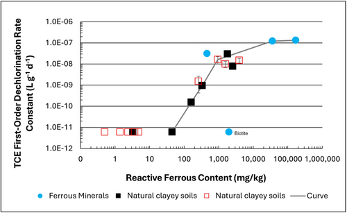
Figure 1: First-order rate constants for abiotic reductive dechlorination of TCE under anaerobic conditions. Circles are data from Schaefer
et al., 2021
[4], filled squares from Schaefer
et al., 2018
[5], and Schaefer
et al., 2017
[6], and open squares from Schaefer
et al., 2025
[1].
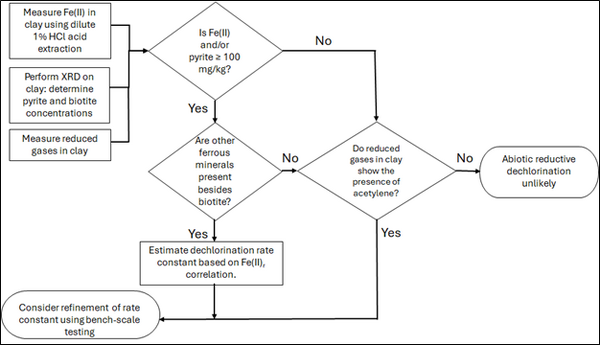
Figure 2: Flowchart diagram of field screening procedures
The recommended approach builds upon the methodology and findings of a recent study[1], emphasizing field-based and analytical techniques to quantify abiotic first-order reductive dechlorination rate constants for PCE and TCE in clayey soils under anoxic conditions. Key components of this evaluation are listed below:
- Zone Identification: The focus of the investigation should be to delineate clayey zones adjacent to hydraulically conductive zones.
- Ferrous Mineral Quantification: Assess ferrous mineral context in clay via 1% HCl extraction at ambient temperature over a 10-minute interval.
- Mineralogical Characterization: Conduct XRD analysis with the specific intent of identifying the presence of pyrite and biotite.
- Reduced Gas Analysis: Measurement of reduced gases such as acetylene, ethene, and ethane concentrations in clay samples. Gas-tight sampling devices (e.g., En Core® soil samplers by En Novative Technologies, Inc.) should be used to ensure sample integrity during collection and transport.
Clay samples should be collected within a few centimeters of the high-permeability interface, with optional additional sampling further inward. For mineralogical analysis, a defined interval may be collected and subsequently subsampled. To preserve sample integrity, exposure to air should be minimized during collection, transport, and handling. Homogenization should occur within an anaerobic chamber, and if subsamples are required for external analysis, they must be shipped in gas-tight, anaerobic containers.
Estimation of the abiotic reductive first-order rate constant for PCE and TCE is based on the “reactive” ferrous content in the clay. Reactive ferrous content (Fe(II)r) is estimated as shown in Equation 1:
- Equation 1: Fe(II)r = DA + XRDpyr - XRDbiotite
where DA is the ferrous content from the dilute acid (1% HCl) extraction, XRDpyr is the pyrite content from XRD analysis, and XRDbiotite is the biotite content from XRD analysis[1].
Abiotic dechlorination is unlikely to contribute to mitigating contaminant back-diffusion when reactive ferrous iron (Fe(II)r) concentrations are below 100 mg/kg (Figure 1). For Fe(II)r above 100 mg/kg, the first-order rate constant for PCE and TCE reductive dechlorination can be estimated using the correlation shown in Figure 1[5][7]. The rate constant exhibits a strong positive correlation with the logarithm of reactive Fe(II) content (Pearson’s r = 0.82), with a slope of 4.7 × 10⁻⁸ L g⁻¹ d⁻¹ (log mg kg⁻¹)⁻¹.
Figure 2 presents a decision flowchart designed to evaluate the significance and extent of abiotic reductive dechlorination. By applying Equation 1 to the dilute acid extractable Fe(II) plus measured mineral species data from clay samples, the reactive ferrous iron content (Fe(II)r) can be quantified, enabling a streamlined assessment of the extent to which abiotic processes are contributing to the mitigation of contaminant back-diffusion.
If Fe(II)r is ≥ 100 mg/kg, a first-order dechlorination rate constant can be estimated and subsequently used within a contaminant fate and transport model. However, if acetylene is detected in the clay, even with Fe(II)r less than 100 mg/kg, then bench-scale testing using methods similar to those described in a recent study[1] is recommended, as such results would likely be inconsistent with those shown in Figure 1, suggesting some other mechanism might be involved, or that the system mineralogy might be more complex than anticipated. Even if Fe(II)r ≥ 100 mg/kg, confirmatory bench-scale testing may be conducted for additional verification and to refine estimation of the abiotic dechlorination rate constant.
Summary and Recommendations
The approach outlined above is intended to serve as a generalized guide for practitioners and site managers to cost-effectively determine the extent to which beneficial abiotic reductive dechlorination reactions are likely occurring in low permeability (e.g., clayey) zones. This approach may be contraindicated if co-contaminants are present. It is currently unclear whether other classes of potentially reactive chemicals, such as trinitrotoluene (TNT) or chlorinated ethanes, could interact competitively with PCE and TCE.
In addition, it remains unclear how other classes of compounds such as per- and polyfluoroalkyl substances (PFAS) may interact or sorb with ferrous minerals and potentially inhibit abiotic dechlorination reactions. Coupling these recommended activities with conventional site investigation tasks would provide an opportunity to perform many of the up-front screening activities with minimal additional project costs. It is important to note that the guidance proposed herein pertains to particularly low permeability media. Sites with complex or varying lithology, where the mineralogy and/or redox conditions may vary, might require evaluation of multiple samples to provide appropriate site-wide information.
References
- ^ 1.0 1.1 1.2 1.3 1.4 Schaefer, C.E., Tran, D., Nguyen, D., Latta, D.E., Werth, C.J., 2025. Evaluating Mineral and In Situ Indicators of Abiotic Dechlorination in Clayey Soils. Groundwater Monitoring and Remediation, 45(2), pp. 31-39. doi: 10.1111/gwmr.12709
- ^ Falta, R., and Wang, W., 2017. A semi-analytical method for simulating matrix diffusion in numerical transport models. Journal of Contaminant Hydrology, 197, pp. 39-49. doi: 10.1016/j.jconhyd.2016.12.007 Open Access Manuscript
- ^ Kulkarni, P.R., Adamson, D.T., Popovic, J., Newell, C.J., 2022. Modeling a well-charactized perfluorooctane sulfate (PFOS) source and plume using the REMChlor-MD model to account for matrix diffusion. Journal of Contaminant Hydrology, 247, Article 103986. doi: 10.1016/j.jconhyd.2022.103986 Open Access Manuscript
- ^ Schaefer, C.E., Ho, P., Berns, E., Werth, C., 2021. Abiotic dechlorination in the presence of ferrous minerals. Journal of Contaminant Hydrology, 241, 103839. doi: 10.1016/j.jconhyd.2021.103839 Open Access Manuscript
- ^ 5.0 5.1 Schaefer, C.E., Ho, P., Berns, E., Werth, C., 2018. Mechanisms for abiotic dechlorination of trichloroethene by ferrous minerals under oxic and anoxic conditions in natural sediments. Environmental Science and Technology, 52(23), pp.13747-13755. doi: 10.1021/acs.est.8b04108
- ^ Schaefer, C.E., Ho., Gurr, C., Berns, E., Werth, C., 2017. Abiotic dechlorination of chlorinated ethenes in natural clayey soils: impacts of mineralogy and temperature. Journal of Contaminant Hydrology, 206, pp. 10-17. doi: 10.1016/j.jconhyd.2017.09.007 Open Access Manuscript
- ^ Borden, R.C., Cha, K.Y., 2021. Evaluating the impact of back diffusion on groundwater cleanup time. Journal of Contaminant Hydrology, 243, Article 103889. doi: 10.1016/j.jconhyd.2021 Open Access Manuscript
See Also

