File list
This special page shows all uploaded files.
| Date | Name | Thumbnail | Size | User | Description | Versions |
|---|---|---|---|---|---|---|
| 14:21, 17 April 2018 | Folkes - 2002. Efficacy of sub-slab depressurization for mitigation of VI.pdf (file) | 201 KB | Debra Tabron | Folkes, D.J. and Kurz, D.W., 2002. Efficacy of sub-slab depressurization for mitigation of vapor intrusion of chlorinated organic compounds. Proceedings of Indoor Air. | 1 | |
| 14:18, 17 April 2018 | USEPA-2010. Temporal Variaiton of VOCs in Soils from GW.PDF (file) | 8.64 MB | Debra Tabron | United States Environmental Protection Agency (USEPA), 2010. Temporal Variation of VOCs in Soils From Groundwater to the Surface/Subslab. U.S. Environmental Protection Agency, Washington, DC, EPA/600/R-10/118, 143 pp. | 1 | |
| 09:59, 17 April 2018 | DON - 2015. A Quantitative Decision...Tech Rpt TR-NAVFAC-EXWC-EV-1603.pdf (file) | 15.72 MB | Debra Tabron | Department of the Navy (DON), 2015. A Quantitative Decision Framework for Assessing Navy Vapor Intrusion Sites. Technical Report TR-NAVFAC-EXWC-EV-1603. | 1 | |
| 09:37, 17 April 2018 | DiGiulio - 2006. Assessment of Vapor Intrusion in Homes...EPA-600-R-05-147.pdf (file) | 7.06 MB | Debra Tabron | DiGiulio, D., Paul, C., Cody, R., Willey, R., Clifford, S., Kahn, P., Mosley, R., Lee, A. and Christensen, K., 2006. Assessment of vapor intrusion in homes near the Raymark Superfund site using basement and sub-slab air samples. EPA/600/R-05/147. | 1 | |
| 11:55, 17 February 2017 | Figure3.gif (file) |  |
10.56 MB | Astenger | 1 | |
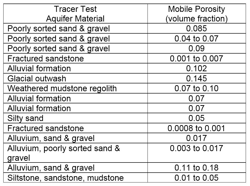
| 10:23, 13 February 2017 | Newell-Article 1-Table2r2.jpg (file) |  |
153 KB | Astenger | 2 | |
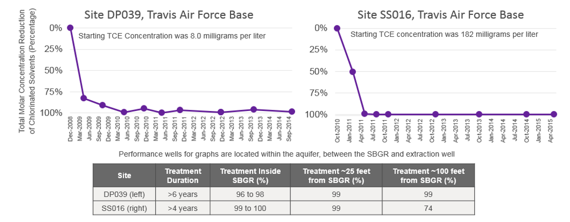
| 16:55, 1 February 2017 | Gamlin SBGR Figure 2.PNG (file) |  |
125 KB | Debra Tabron | Figure 2. SBGR performance observations for two chlorinated solvent sites in California | 1 |
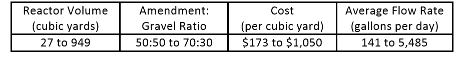
| 16:54, 1 February 2017 | Gamlin SBGR Table 1.PNG (file) | 14 KB | Debra Tabron | Table 1. SBGR Construction and Cost Details | 1 | |
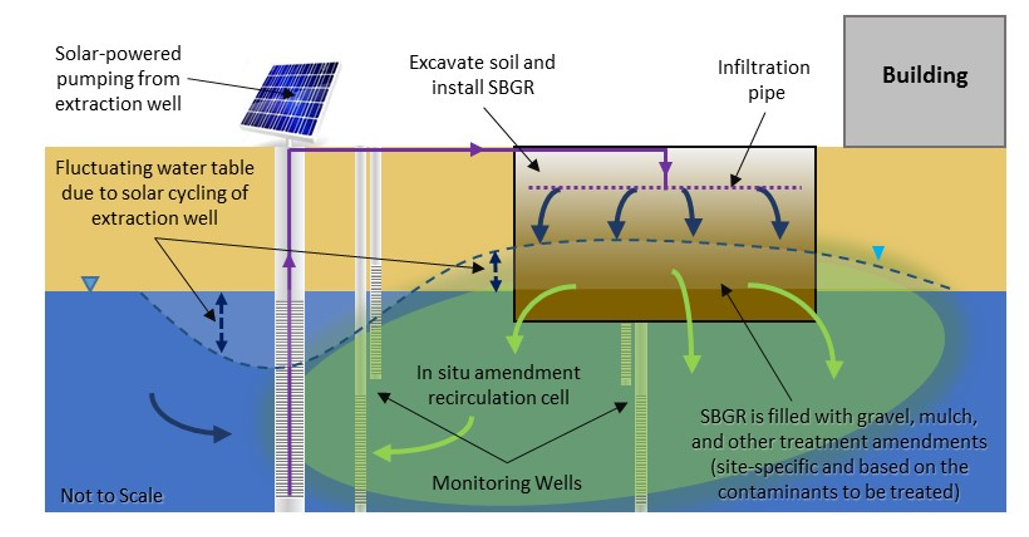
| 16:53, 1 February 2017 | Gamlin SBGR Figure 1.PNG (file) |  |
561 KB | Debra Tabron | Figure 1. Typical subgrade biogeochemical reactor (SBGR) layout. | 1 |
| 19:58, 31 January 2017 | Slater Intro Fig3 new2.jpg (file) |  |
4.97 MB | Jbarnes | 1 | |
| 19:53, 31 January 2017 | Slater Intro Table3 new.jpg (file) |  |
1.04 MB | Jbarnes | 1 | |
| 19:52, 31 January 2017 | Slater Intro Fig3 new.jpg (file) |  |
4.97 MB | Jbarnes | 1 | |
| 14:17, 31 January 2017 | Slater CaseStudies Fig3.jpg (file) |  |
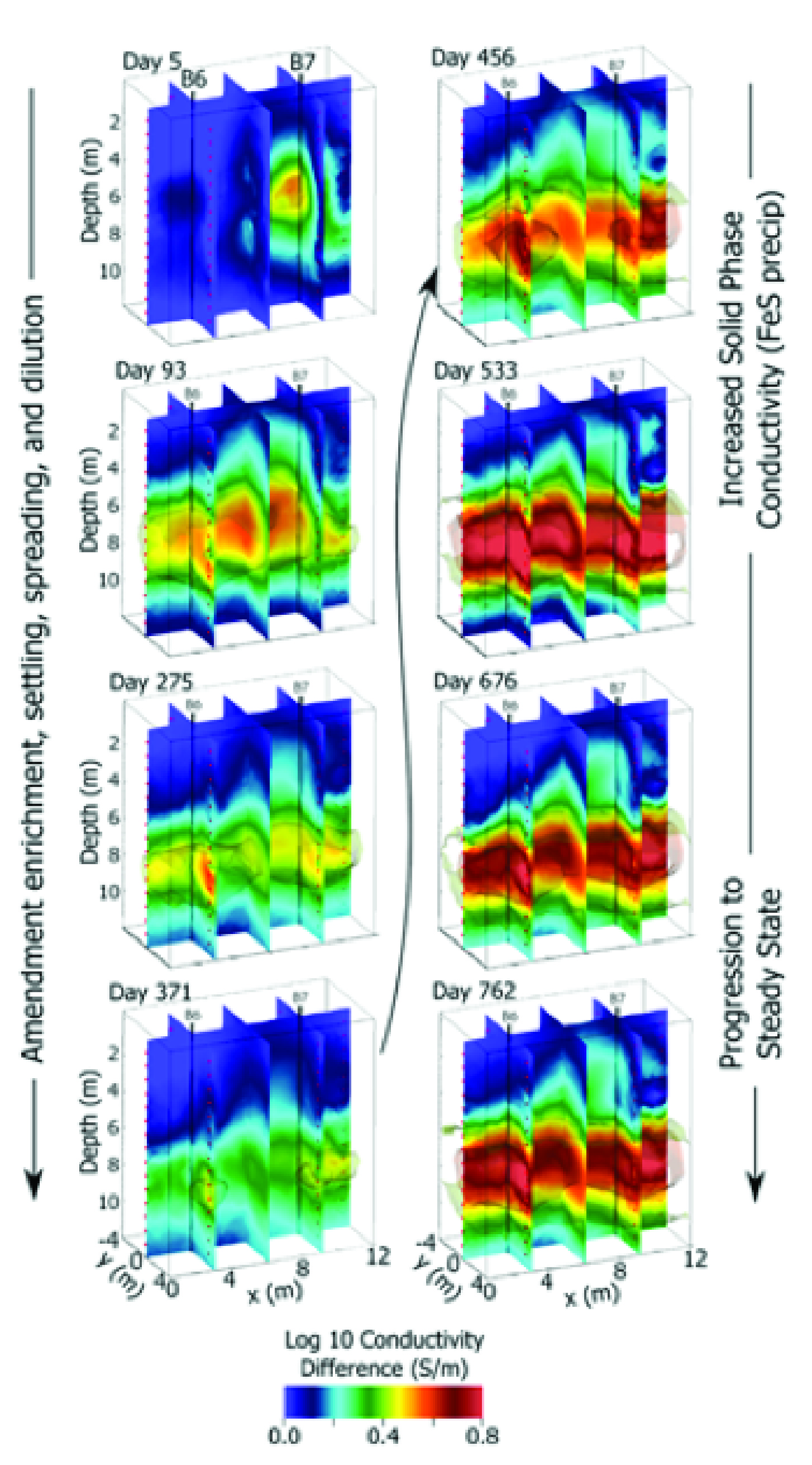
2.5 MB | Debra Tabron | Figure 3. Example 3D time-lapse ERT images showing bioamendment emplacement and movement, seen as increased bulk electrical conductivity (first column), followed by later increase in bulk conductivity arising from FeS precipitation resulting from micro... | 1 |
| 14:16, 31 January 2017 | Slater-Article 2-Figure 2.PNG (file) |  |
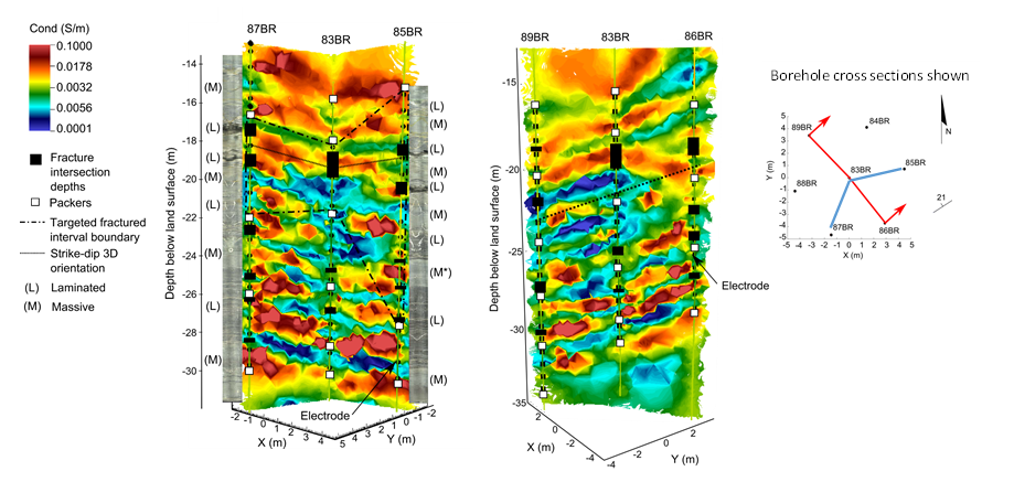
353 KB | Debra Tabron | Figure 2. High-resolution 3D cross-borehole electrical imaging of contaminated fractured rock at the former Naval Air Warfare Center in New Jersey. Two panels of the 3D volume of earth imaged are shown for comparison. Acoustic televiewer images recorde... | 1 |
| 14:15, 31 January 2017 | Slater-Article 2-Figure 1.PNG (file) |  |
630 KB | Debra Tabron | Figure 1. Resistivity imaging at the 300 Area of the Hanford Facility, Richland, WA. (a) location of 2D resistivity survey lines. (b) selected 2D resistivity profiles (locations in part a) showing imaging of variations in depth to the Hanford-Ringold c... | 1 |
| 10:32, 31 January 2017 | Slater Intro Table3.jpg (file) |  |
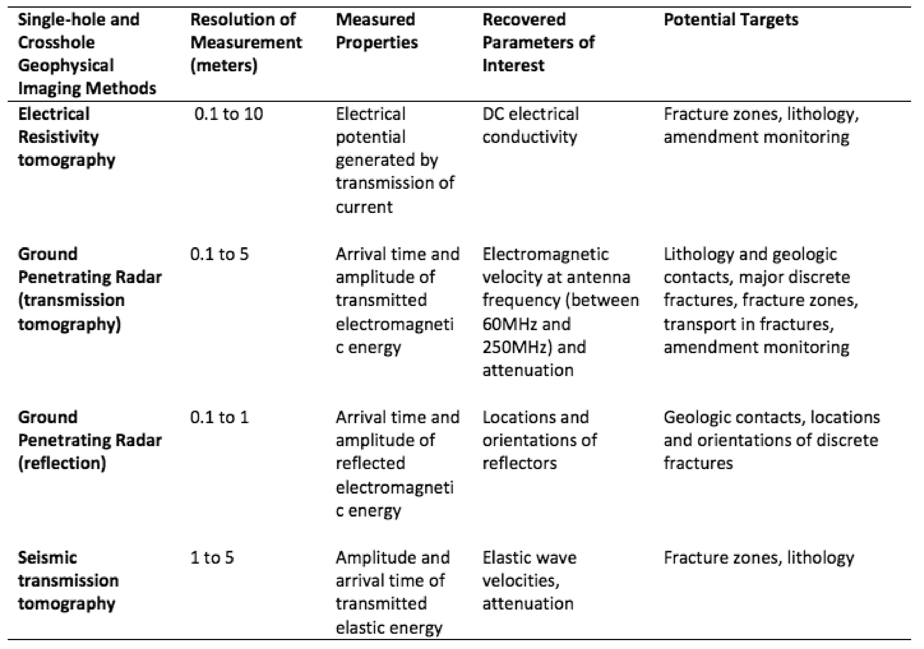
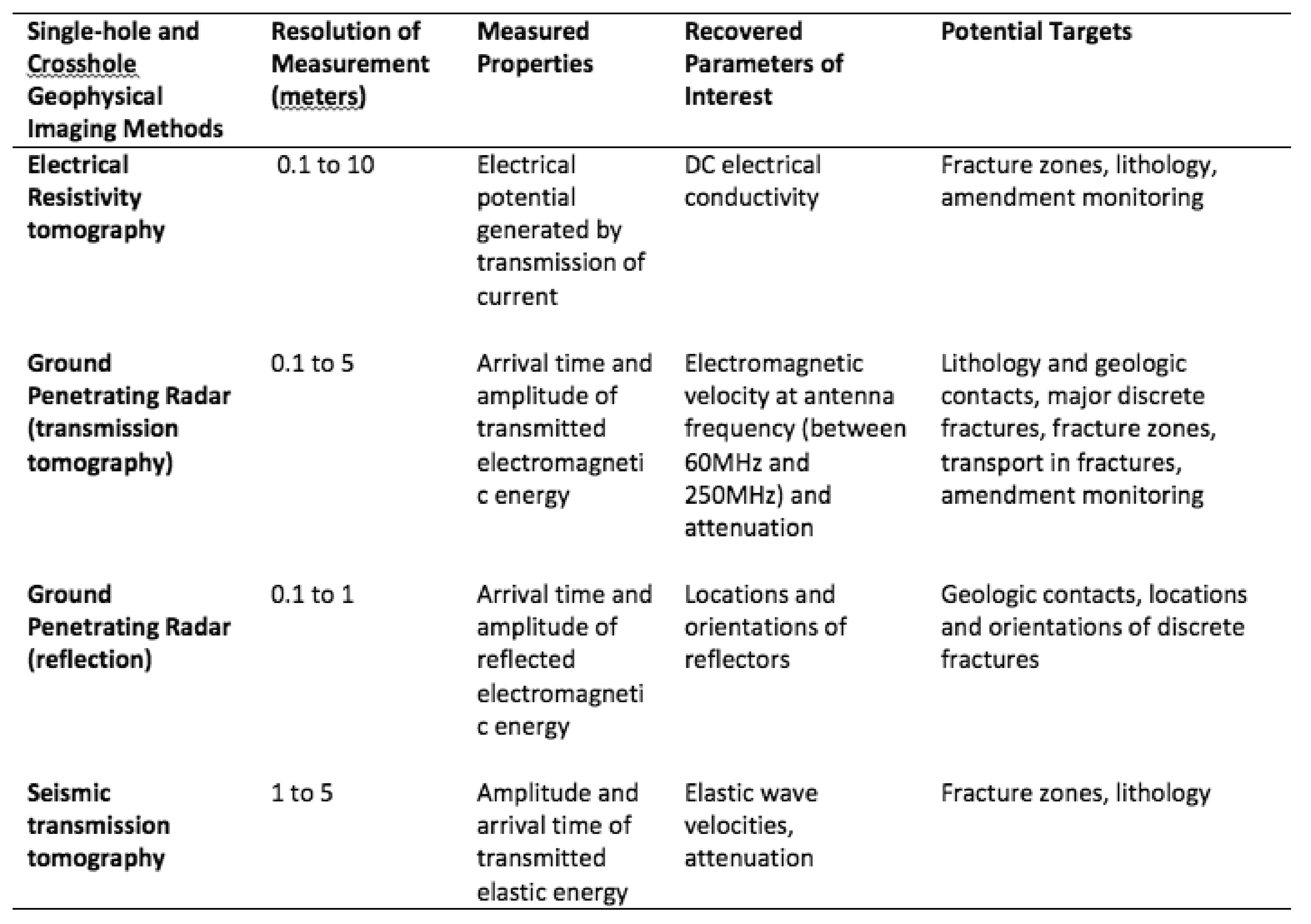
1.04 MB | Debra Tabron | Table 3. Details of four single-hole and crosshole geophysical imaging methods with potential application to contaminated sites. The lateral extent and depth of the surveyed region, and resolution of the measurement, are all typical values for environm... | 1 |
| 10:30, 31 January 2017 | Slater Intro Table2.jpg (file) |  |
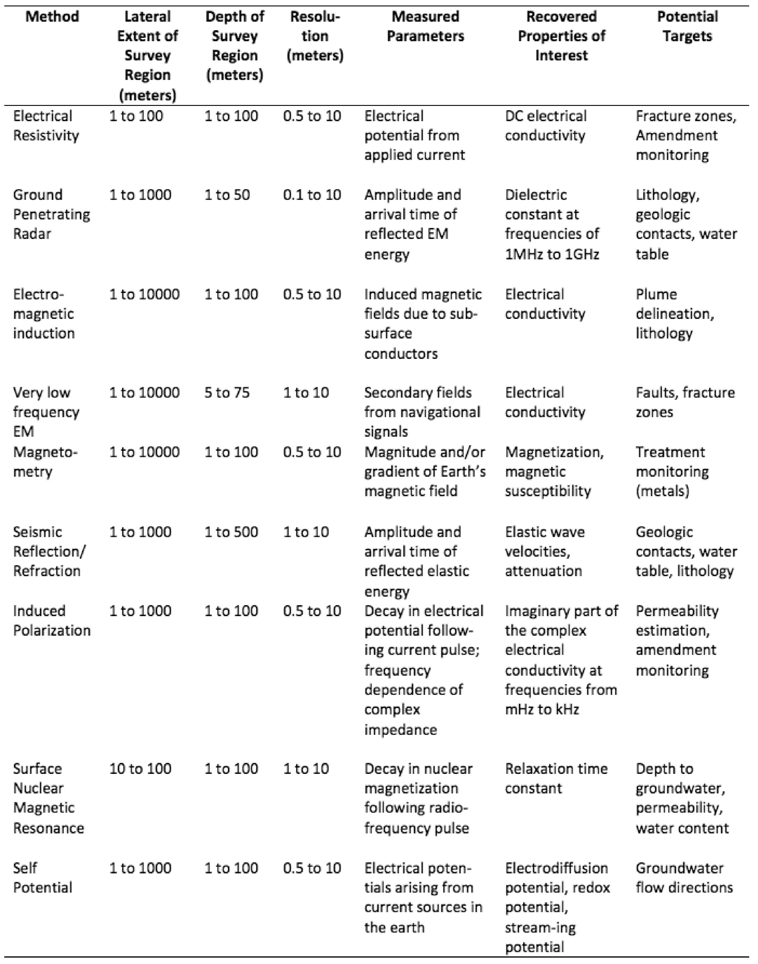
1.4 MB | Debra Tabron | Table 2. Surface-based geophysical methods commonly used at remediation sites. The extent and depth of the survey region and the resolution are all approximate ranges. The measured parameters can be derived directly from the acquired data. The recovere... | 1 |
| 10:29, 31 January 2017 | Slater Intro Table1.jpg (file) |  |
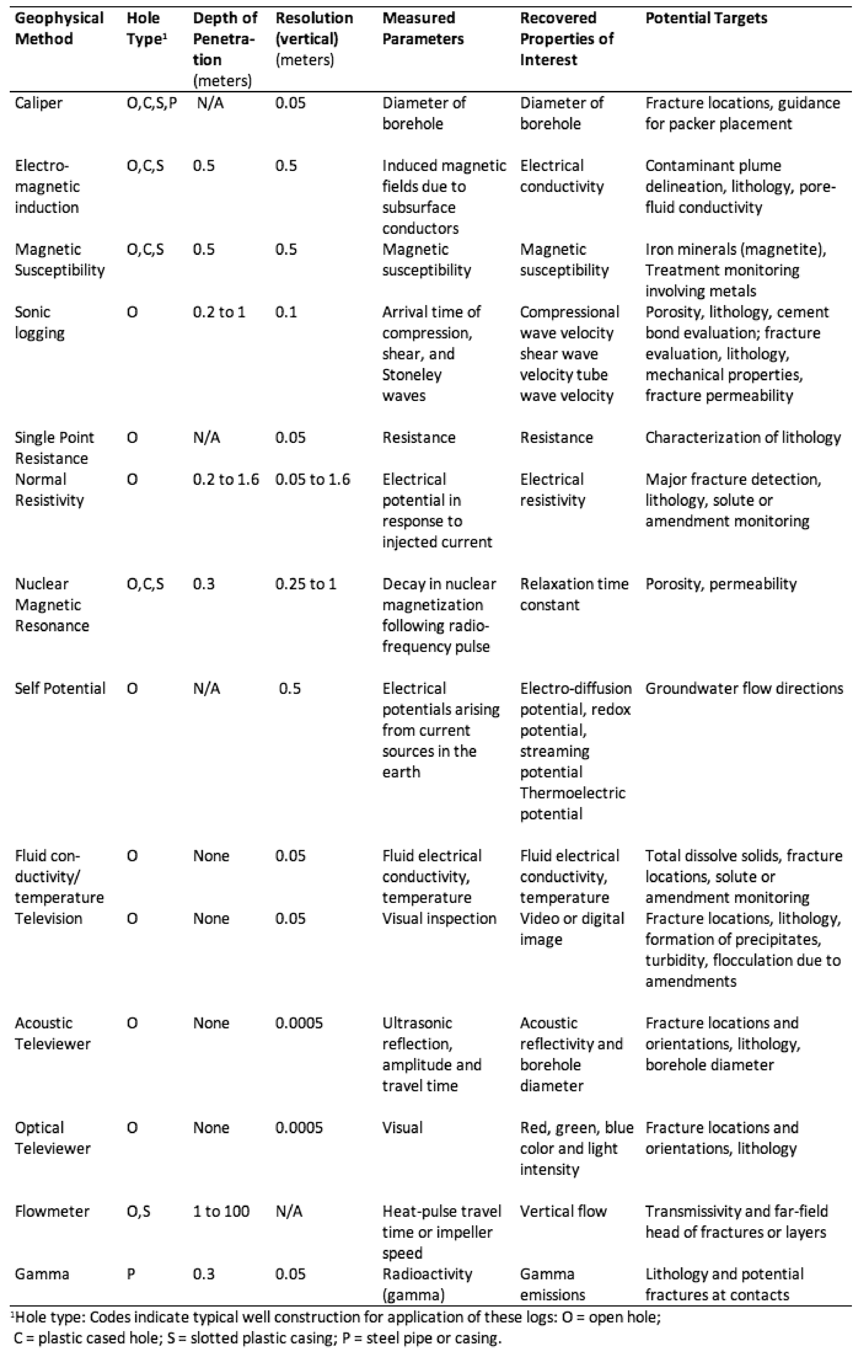
2.24 MB | Debra Tabron | Table 1. Details of borehole geophysical logging methods commonly used at remediation sites. The lateral depth of penetration into the formation and resolution of the measurement are approximate ranges for site investigation. The measured parameters ca... | 1 |
| 10:27, 31 January 2017 | Slater Intro Fig4.PNG (file) |  |
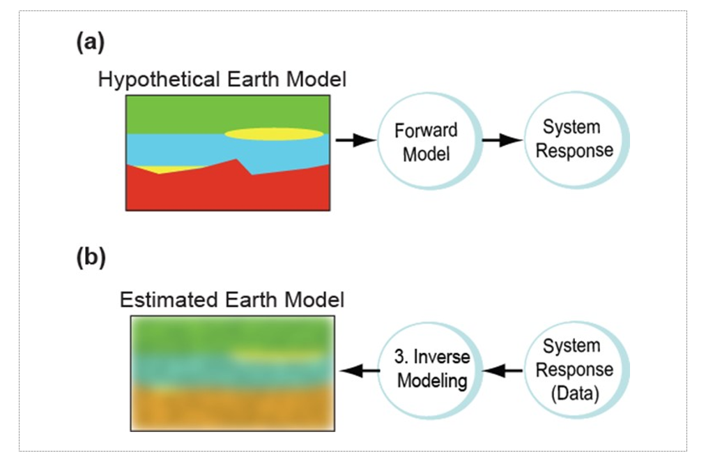
282 KB | Debra Tabron | Figure 4. Schematic explanation of the concepts of (a) forward modeling and (b) inverse modeling. | 1 |
| 10:23, 31 January 2017 | Slater Intro Fig3.jpg (file) |  |
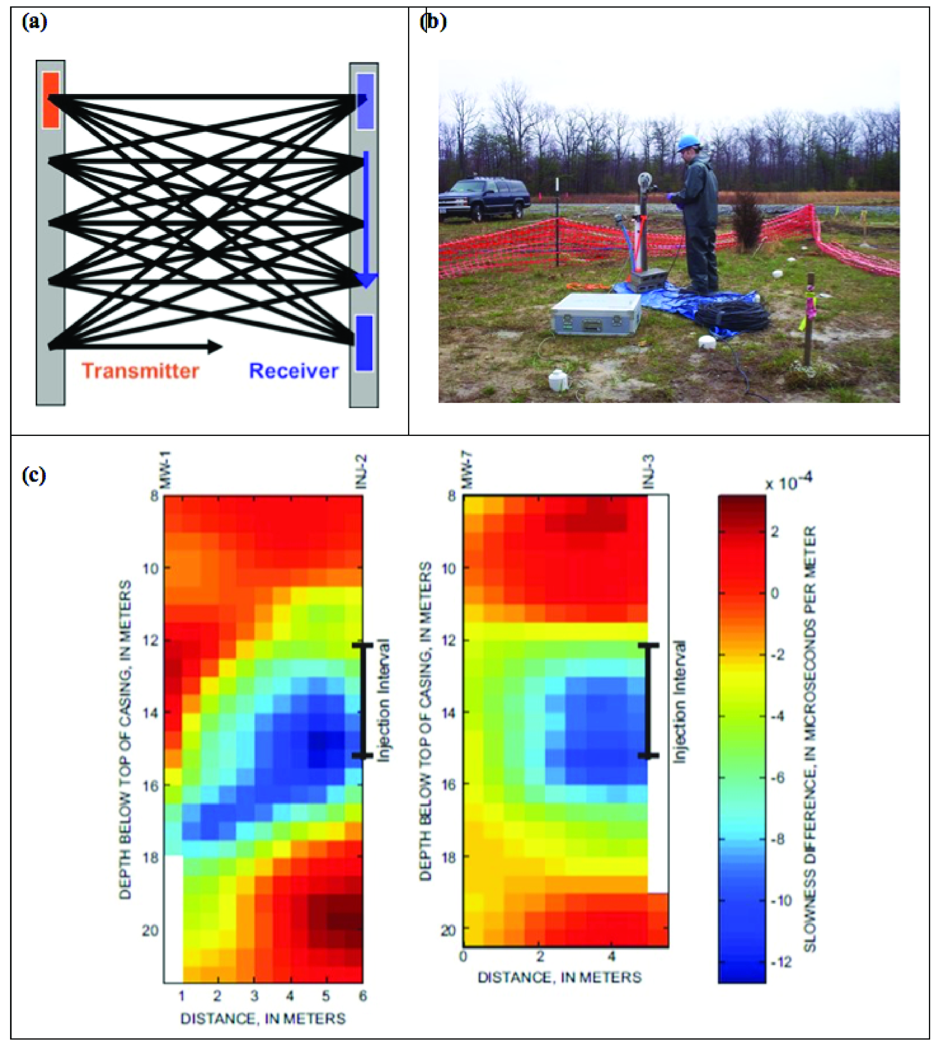
3.25 MB | Debra Tabron | Figure 3. Example cross-borehole method. (a) Schematic crosshole radar tomography, in which a transmitting antenna is moved vertically in one well, and a receiver antenna is moved vertically in another well. High-frequency electromagnetic waves are tra... | 1 |
| 09:52, 31 January 2017 | Slater Intro Fig2.jpg (file) |  |
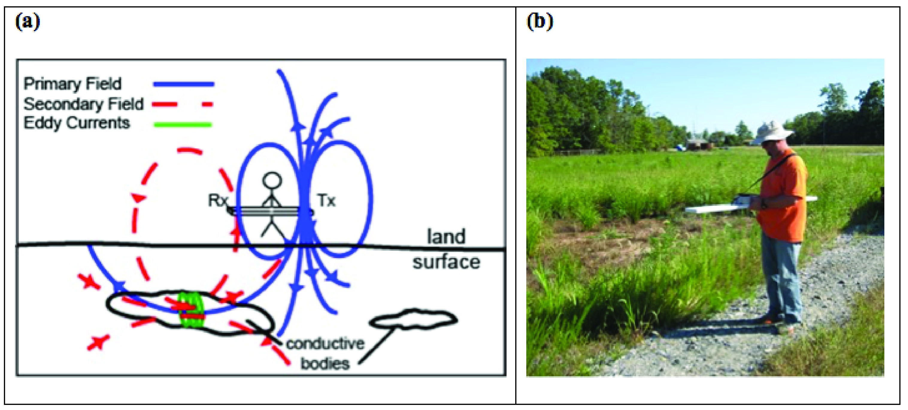
2.69 MB | Debra Tabron | Figure 2. Example of a surface-based geophysical method. (a) Schematic diagram of an electromagnetic induction tool in operation, which comprises a transmitter (Tx) and receiver (Rx) to respectively produce a primary electromagnetic field and measure a... | 1 |
| 09:50, 31 January 2017 | Slater Intro Fig1.jpg (file) |  |
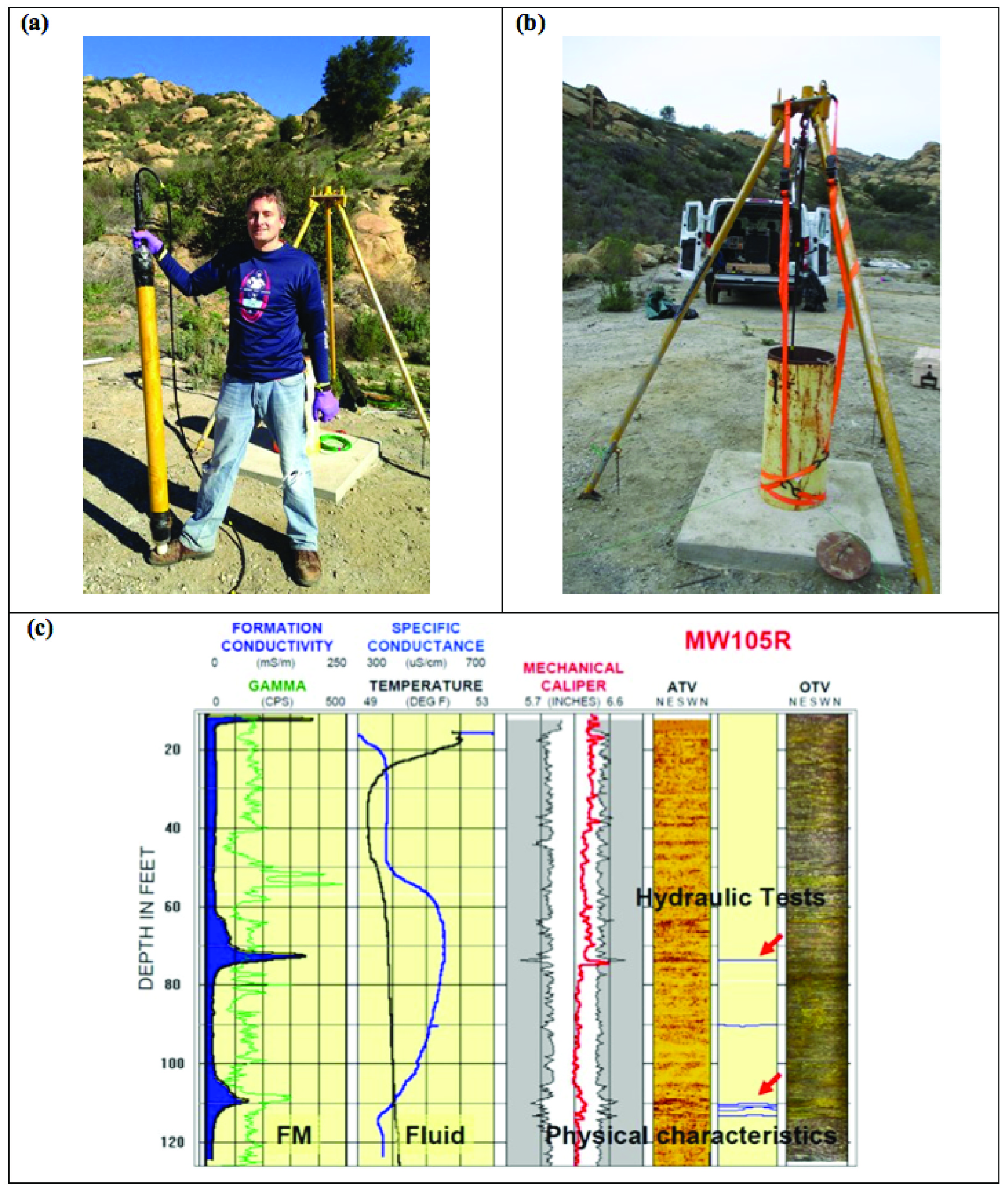
3.39 MB | Debra Tabron | Figure 1. Example borehole logging equipment and log panel from the U. Connecticut Landfill in which major fractures appear in multiple logs for well MW105R at ~110 ft, 90 ft, and 75 ft depths (after Johnson et al., 2002.(a) Borehole tool outside of the | 1 |
| 14:49, 30 January 2017 | Krug-Article 2-Figure 3.PNG (file) |  |
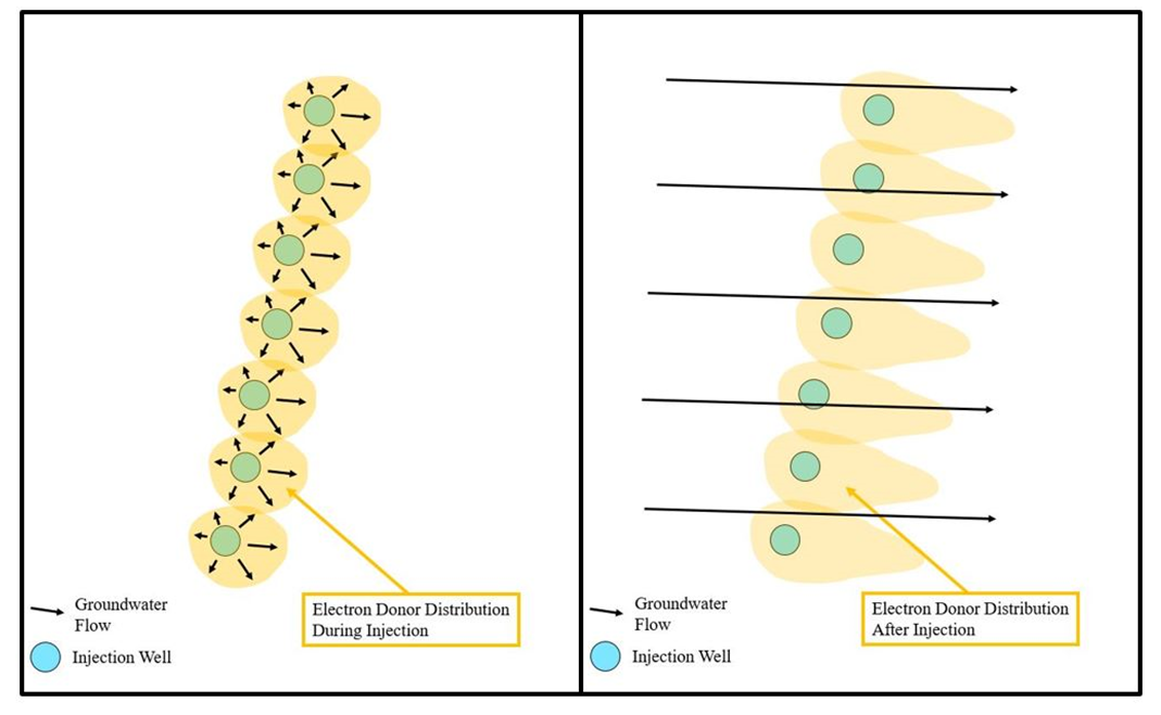
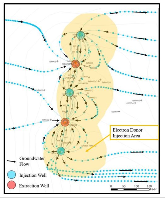
344 KB | Debra Tabron | Figure 3. Example of electron donor distribution during (left panel) and after (right panel) injection. | 1 |
| 14:48, 30 January 2017 | Krug-Article 2-Figure 2.PNG (file) |  |
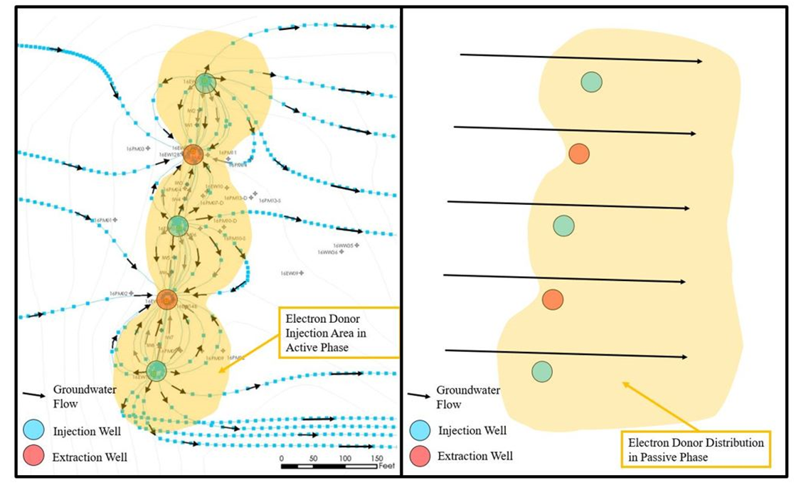
673 KB | Debra Tabron | Figure 2. Electron donor distribution during the active semi-passive amendment injection phase (left panel) and the passive phase (right panel). | 1 |
| 14:47, 30 January 2017 | Krug-Article 2-Figure 1.PNG (file) |  |
577 KB | Debra Tabron | Figure 1. Example electron donor distribution during active amendment injection. | 1 |
| 11:41, 30 January 2017 | Johnson-2002-Borehole-Geophysical Investigation.pdf (file) | 3.28 MB | Astenger | 1 | ||
| 09:14, 30 January 2017 | Denham-Article 4-Figure 1.PNG (file) |  |
249 KB | Debra Tabron | Figure 1. Example of an Attenuation Conceptual Model for metals contamination | 1 |
| 20:42, 26 January 2017 | Freedman BRP Fig2.jpg (file) |  |
1.74 MB | Jbarnes | 1 | |
| 20:35, 26 January 2017 | Freedman BRP Fig1.jpg (file) | 1.35 MB | Jbarnes | 1 | ||
| 20:34, 26 January 2017 | Freedman BRP EQ1.jpg (file) | 33 KB | Jbarnes | 1 | ||
| 11:17, 25 January 2017 | Edwards Article 1-figure 3.PNG (file) |  |
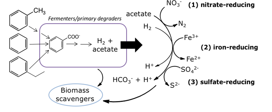
74 KB | Debra Tabron | Figure 3. Conceptual model for syntrophic anaerobic degradation of benzene and alkylbenzenes. Acetate and H2 are consumed in reactions 1, 2, and 3, keeping the fermentation reaction energetically favorable. When external electron acceptors (e.g., nitra... | 1 |
| 11:15, 25 January 2017 | Edwards Article 1-figure 2.PNG (file) |  |
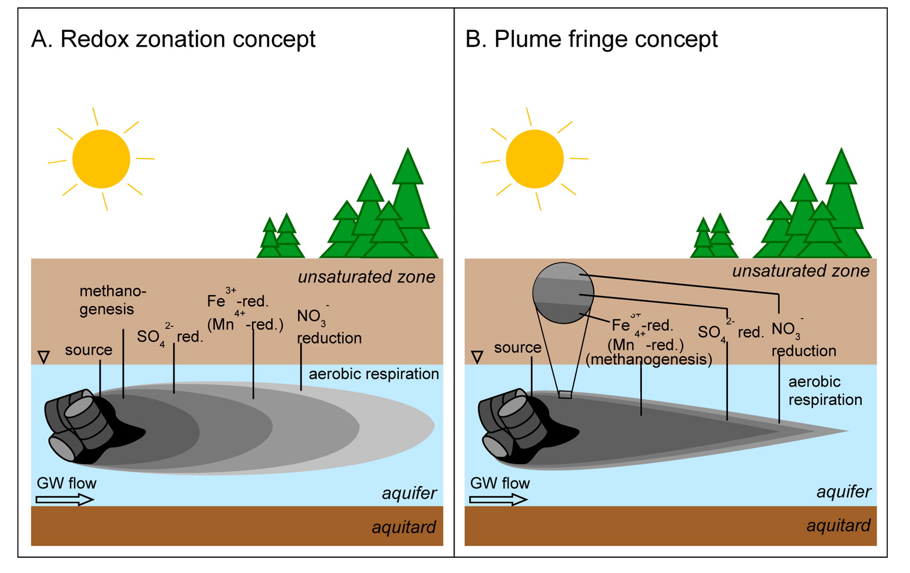
241 KB | Debra Tabron | Figure 2. Comparison of the longitudinal redox zonation concept (A) and the plume fringe concept (B). Both concepts describe the spatial distribution of electron acceptors and respiration processes in a hydrocarbon contaminant plume. (B) Iron(III) redu... | 1 |
| 11:12, 25 January 2017 | Edwards Article 1-figure 1.PNG (file) |  |
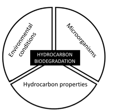
58 KB | Debra Tabron | Figure 1. Components of hydrocarbon biodegradation. Understanding and facilitating biodegradation at a contaminated site requires knowledge of the environmental conditions, compound properties, and microorganisms present (Adapted after Sutherson, 1999) | 1 |
| 16:27, 24 January 2017 | USEPA-1994-How to evalutate alternative cleanup tech for UST Sites.pdf (file) | 1.8 MB | Debra Tabron | United States Environmental Protection Agency, 1994. How to evaluate alternative cleanup technologies for underground storage tank sites | 1 | |
| 12:14, 24 January 2017 | ATSDR-1999-Tox profile for TPH.pdf (file) | 8.31 MB | Debra Tabron | Agency for Toxic Substances and Disease Registry, 1999. Toxicological profile for total petroleum hydrocarbons (TPH). Accessed December 1, 2016 from | 1 | |
| 12:22, 23 January 2017 | Denham-Article 3-Table 2.PNG (file) |  |
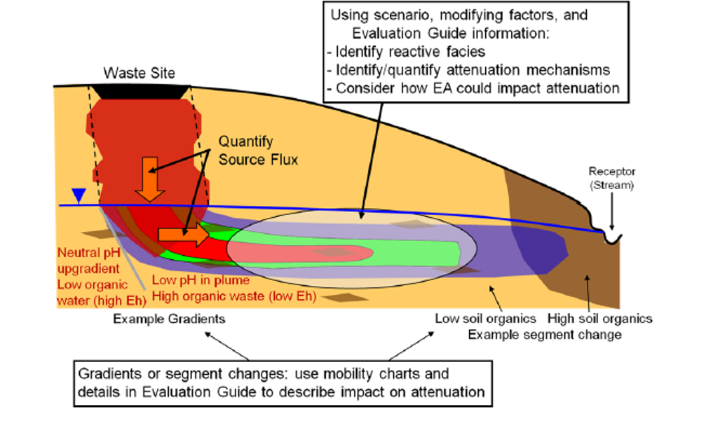
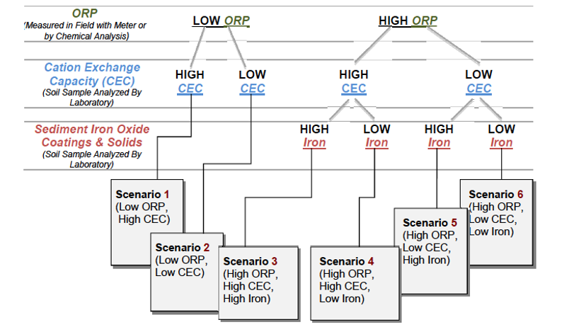
136 KB | Debra Tabron | Table 2. Six Scenarios for Evaluating Inorganic Monitored Natural Attenuation | 1 |
| 12:20, 23 January 2017 | Denham-Article 3-Table 1.PNG (file) |  |
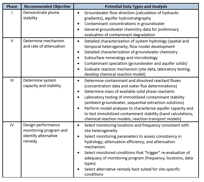
55 KB | Debra Tabron | Table 1. Tiered four-phase approach to demonstrating MNA for inorganic compounds | 1 |
| 12:19, 23 January 2017 | Denham-Article 3-Figure 2.PNG (file) |  |
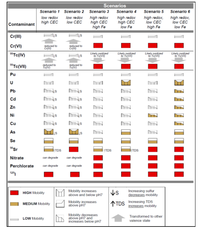
228 KB | Debra Tabron | Figure 2. Summary of inorganic contaminant mobility for 4 < pH < 9 for six scenarios | 1 |
| 12:18, 23 January 2017 | Denham-Article 3-Figure 1.PNG (file) |  |
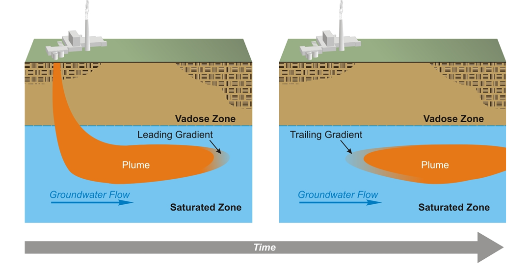
230 KB | Debra Tabron | Figure 1. Typical contaminant plume evolution in an aquifer showing leading and trailing gradients. | 1 |
| 12:16, 19 January 2017 | Freedman A 1 Fig 4.PNG (file) |  |
5 KB | Debra Tabron | 1 | |
| 11:36, 19 January 2017 | Freedman A 1 Fig 3.PNG (file) |  |
5 KB | Debra Tabron | 1 | |
| 10:45, 19 January 2017 | Freedman Article 1 Figure 6.PNG (file) |  |
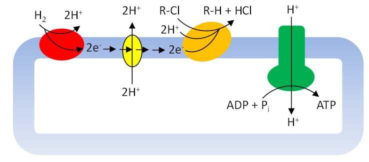
21 KB | Debra Tabron | Figure 6. Schematic representation of a microbial cell carrying out organohalide respiration. Blue shape = the cell membrane; red oval = hydrogenase; yellow oval = electron carrier and proton translocation; orange oval = reductive dehalogenase; green s... | 1 |
| 10:42, 19 January 2017 | Freedman Article 1 Figure 5.PNG (file) |  |
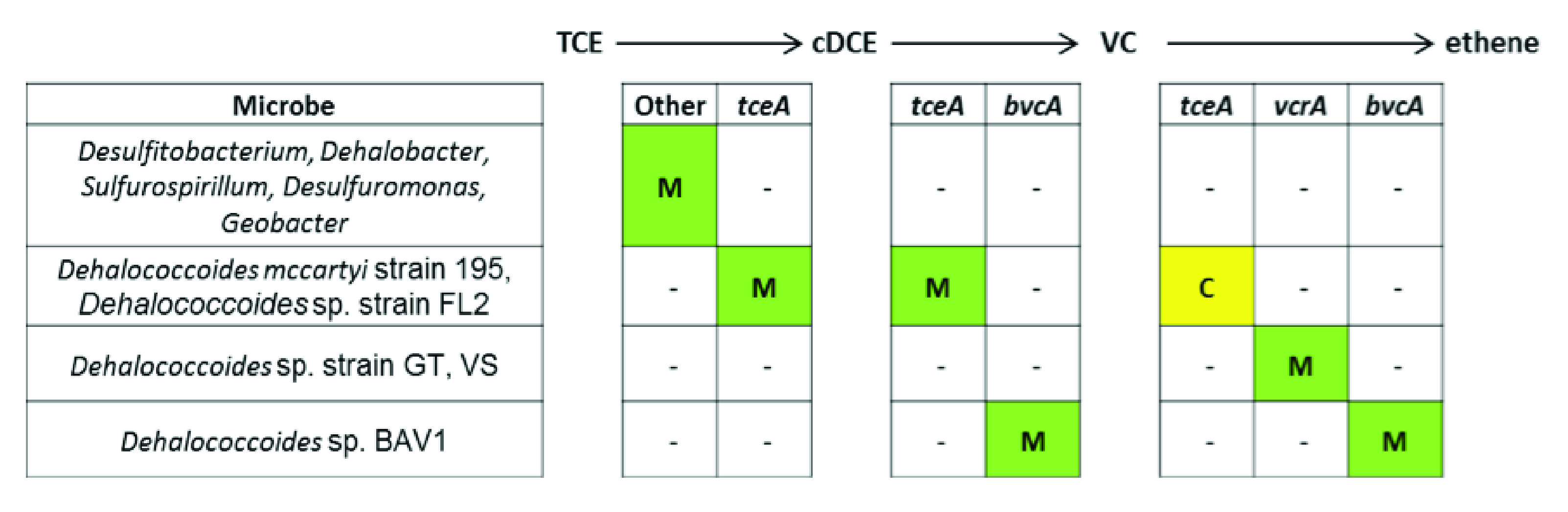
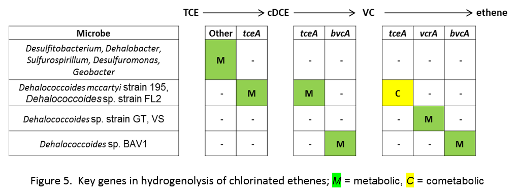
60 KB | Debra Tabron | Figure 5. Key genes in hydrogenolysis of chlorinated ethenes; M = metabolic, C = cometabolic | 1 |
| 10:39, 19 January 2017 | Freedman Article 1 Figure 4.PNG (file) |  |
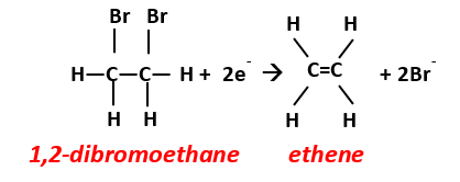
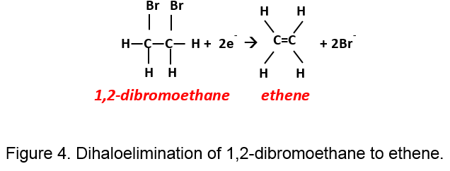
10 KB | Debra Tabron | Figure 4. Dihaloelimination of 1,2-dibromoethane to ethene. | 1 |
| 10:10, 19 January 2017 | Freedman Article 1 Figure 2.PNG (file) |  |
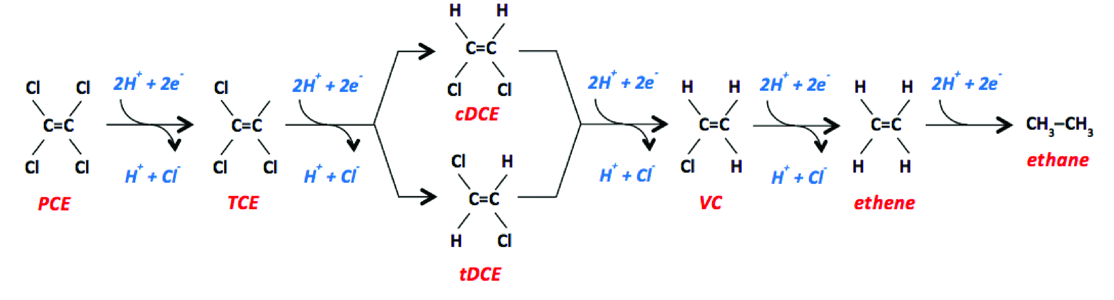
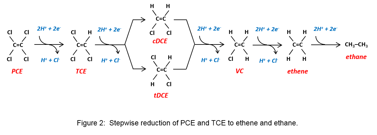
27 KB | Debra Tabron | Figure 2. Stepwise reduction of PCE and TCE to ethene and ethane | 1 |
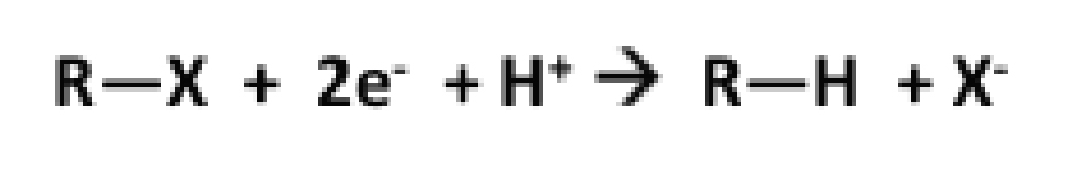
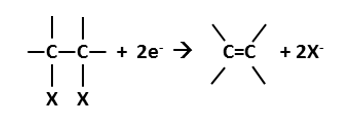
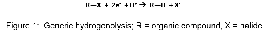
| 10:07, 19 January 2017 | Freedman Article 1 Figure 1.PNG (file) | 8 KB | Debra Tabron | Figure 1. Generic hydrogenolysis; R = organic compound, X = halide. | 1 | |
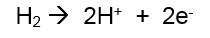
| 10:04, 19 January 2017 | Freedman Article 1 Equation 1.PNG (file) | 962 bytes | Debra Tabron | 1 | ||
| 15:17, 17 January 2017 | Heron Combined Therm Fig3.jpg (file) |  |
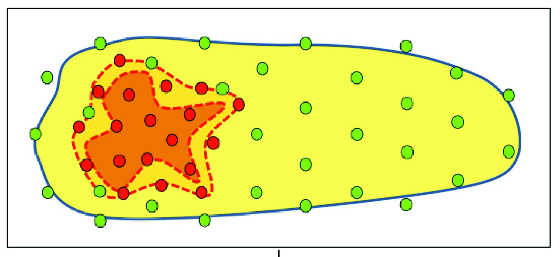
1.03 MB | Debra Tabron | Figure 3. Example combined remedy: Thermal treatment of the source zone combined with bioremediation for treating the transition zone and dissolved plume. Red dots = heaters, green dots = bioremediation injection or extraction wells. | 1 |
| 15:16, 17 January 2017 | Heron Combined Therm Fig2.jpg (file) |  |
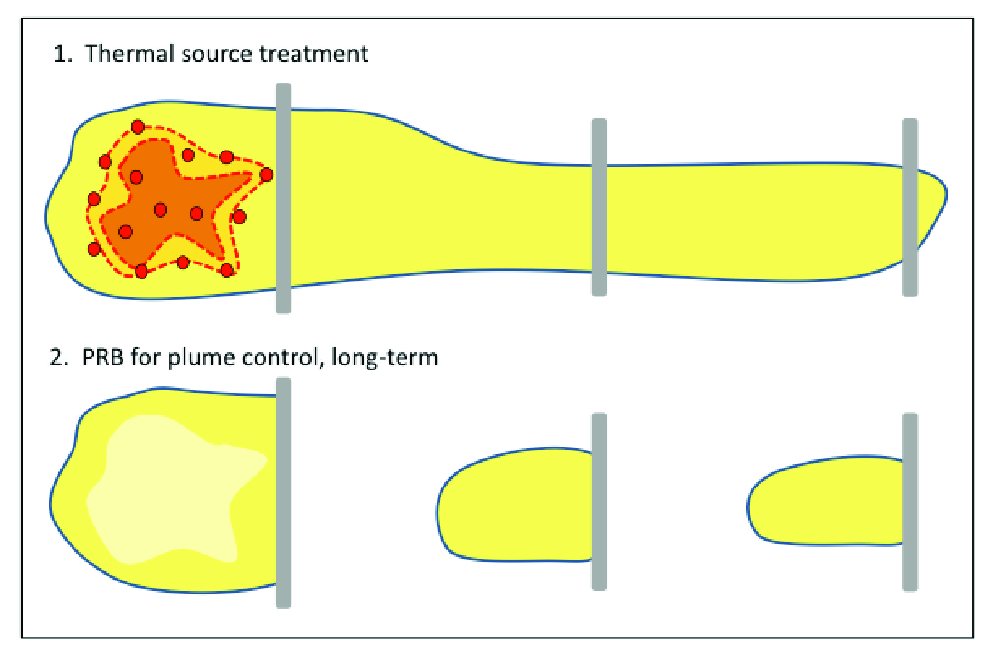
1.14 MB | Debra Tabron | Figure 2. Example combined remedy. Thermal treatment of the source zone combined with permeable reactive barriers for treating a long dissolved plume. Thermal source treatment is implemented in the first year, followed by plume treatment in a period af... | 1 |
| 15:15, 17 January 2017 | Heron Combined therm Table 1.PNG (file) |  |
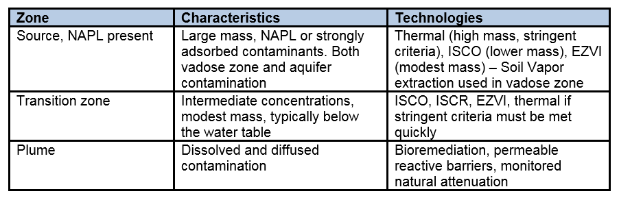
33 KB | Debra Tabron | Table 1. Technologies applied in the different zones of a complex contaminated site. | 1 |