|
|
| Line 3: |
Line 3: |
| | | | |
| | '''Related Article(s)''': | | '''Related Article(s)''': |
| − | *[[Monitored Natural Attenuation (MNA)]] | + | *LNAPL Source Zone Conceptual Models (Coming soon) |
| − | | + | *LNAPL Remediation Technologies (Coming soon) |
| | | | |
| | | | |
| Line 11: |
Line 11: |
| | | | |
| | '''Key Resource(s)''': | | '''Key Resource(s)''': |
| − | *[[media:2002-Newell-Calculation and Use of First-Order Rate Constants for Monitored Natural Attenuation Studies.pdf| Calculation and Use of First-Order Rate Constants for Monitored Natural Attenuation Studies]]<ref name= "Newell2002">Newell, C.J., Rifai, H.S., Wilson, J.T., Connor, J.A., Aziz, J.A., Suarez, M.P., 2002. Calculation and use of first-order rate constants for monitored natural attenuation studies. 28p. EPA/540/S-02/500. [[media:2002-Newell-Calculation and Use of First-Order Rate Constants for Monitored Natural Attenuation Studies.pdf| Report.pdf]]</ref> | + | *[https://lnapl-3.itrcweb.org LNAPL Site Management: LCSM Evolution, Decision Process, and Remedial Technologies]<ref name= "ITRC2018">ITRC, 2018. LNAPL Site Management: LCSM evolution, decision process, and remedial technologies (LNAPL-3). Interstate Technical and Regulatory Council </ref>. Section 3 provides an introductory discussion of LNAPL mobility concepts. |
| − | *[https://www.nas.cee.vt.edu/index.php Natural Attenuation Software (NAS) Version 2.3.3]<ref name= "Widdowson2008">Widdowson, M.A., Mendez, E., Chapelle, F.H., Casey, C.C., 2008. Natural Attenuation Software (NAS) Version 2.3.3. Virginia Polytechnic Institute and State University, the United States Geological Survey, and the United States Naval Facilities Engineering Command. </ref> | + | *[https://www.api.org/oil-and-natural-gas/environment/clean-water/ground-water/lnapl/ldrm API LNAPL Distribution and Recovery Model (LDRM), API 4760] <ref name= "Charbeneau2007">Charbeneau, R.J., 2007. LNAPL Distribution and Recovery Model. Distribution and Recovery of Petroleum Hydrocarbon Liquids in Porous Media. Vol. 1. API Publication 4760. [[media:API2007_LDRM.pdf | Report.pdf]]</ref>. Provides detailed discussion of LNAPL mobility as related to saturation, soil properties and capillary pressure. |
| − | *[[media:2002-Aziz-Biochlor Natural Attenuation Decision Support System Vs 2.2.pdf| BIOCHLOR Natural Attenuation Support System, Version 2.2]]<ref name= "Aziz2002">Aziz, C.E., Newell, C.J. and Gonzales, J.R., 2002. BIOCHLOR Natural Attenuation Decision Support System Version 2.2 User’s Manual Addendum. Groundwater Services, Inc., Houston, Texas for the Air Force Center for Environmental Excellence.[[media:2002-Aziz-Biochlor Natural Attenuation Decision Support System Vs 2.2.pdf| Report.pdf]]</ref> | + | *[https://www.crccare.com/files/dmfile/CRCCARETechnicalreport44_TechnicalmeasurementguidanceforLNAPLnaturalsourcezonedepletion.pdf Technical measurement guidance for LNAPL natural source zone depletion]<ref name= "CRCCARE2018">CRC CARE, 2018. Technical measurement guidance for LNAPL natural source zone depletion. Cooperative Research Centre for Contamination Assessment and Remediation of the Environment, Newcastle, Australia. Technical Report no. 44. 254p [[media:CRCCARE2018_Measurement_Guidance_for_LNAPL_NSZD.pdf | Report.pdf]]</ref>. |
| | + | *Section 6 provides a discussion of compositional changes to LNAPL over time and how to use those changes to calculate natural source zone depletion rates. |
| | | | |
| | ==Introduction== | | ==Introduction== |
| − | Many active remedies are effective at treating higher concentrations of contaminants, but as the contaminant concentrations decrease, the rate of cleanup may slow until it is not significantly different from the rate of cleanup provided by the natural attenuation processes that occur at the site. The United States Environmental Protection Agency (USEPA 1999)<ref> U.S. Environmental Protection Agency (USEPA), 1999. Use of monitored natural attenuation at superfund, RCRA corrective action, and underground storage tank sites. [[media:1999 USEPA- Use of monitored natural attenuation at superfund.pdf| Report.pdf]]</ref> allows the use of [[Monitored Natural Attenuation (MNA) | monitored natural attenuation (MNA)]] to attain the cleanup goals when the site-specific remediation objectives can be attained within a time frame that is reasonable compared to that offered by other more active methods. Many CERCLA<ref>U.S. Environmental Protection Agency (USEAP), 2019a. Summary of the Comprehensive Environmental Response, Compensation, and Liability Act (Superfund)</ref> and RCRA<ref>U.S. Environmental Protection Agency (USEPA), 2019b. Resource Conservation and Recovery Act (RCRA) Laws and Regulations</ref> sites take advantage of this policy. An active remedy is typically used initially to treat high concentrations of contaminants followed by MNA to treat the lower concentrations that remain.
| + | LNAPL can be found in the subsurface in three different states: |
| − | | + | #'''Residual LNAPL''' is trapped and immobile but can undergo composition change and generate dissolved hydrocarbon plumes and/or vapor sources in the unsaturated zones. |
| − | Unfortunately, there is no well-established approach to determine when it is appropriate to discontinue the active remedy. This article reviews available tools and approaches to evaluate a transition to MNA.
| + | #'''Mobile LNAPL''' is LNAPL at greater than the residual saturation which can therefore accumulate in a well where it is potentially recoverable. However, in this state LNAPL saturation is insufficient to drive migration (i.e., the LNAPL body is not expanding). |
| − | The tools and approaches depend on calculations of rate constants for natural attenuation with distance in flowing groundwater or rate constants for attenuation over time in individual monitoring wells. The next section provides some background on first-order constants and how they are extracted from monitoring data.
| + | #'''Migrating LNAPL''' is LNAPL at greater than the residual saturation that expands into previously unimpacted locations over time (e.g., LNAPL appears in a monitoring well that had no previous detections). |
| − | | |
| − | ==Background on Rate Constants ==
| |
| − | | |
| − | A general formula to describe the rate of a chemical reaction is:
| |
| − |
| |
| − | :{|
| |
| − | |-
| |
| − | | '''Equation 1:''' || || <big>''r = k [C]</big><sup> m</sup>''
| |
| − | |-
| |
| − | |where:
| |
| − | |-
| |
| − | | || ''r'' || is the rate of the reaction,
| |
| − | |-
| |
| − | | || ''k''|| is the rate constant,
| |
| − | |-
| |
| − | | || ''C''|| is the concentration of the chemical undergoing the reaction, and
| |
| − | |-
| |
| − | |the exponent || ''m''|| is the order of the reaction.
| |
| − | |}
| |
| − | | |
| − | When the rate of the reaction is proportional to the concentration of the contaminant, the value of ''m'' is 1. Therefore, the reaction is described as a first-order reaction, and the rate constant is described as a first-order rate constant. In Equation 1, concentration could go up or down, but ''k'' is a constant of proportionality for the rate of increase in concentration. The rate constant for attenuation is the negative of ''k''. If the rate of degradation is a fixed value regardless of concentration, the value of ''m'' is 0, and degradation is a zero-order process.
| |
| − | | |
| − | Natural attenuation of concentrations over time in monitoring wells is frequently described by a first-order rate constant, and natural biological or abiotic degradation of contaminants in flowing groundwater is typically also described by a first-order rate constant. Figure 1 provides an example of monitoring data that is described by a first-order rate constant.
| |
| − | | |
| − | [[File:Wilson1w2Fig1.png|thumb|Figure 1. Attenuation of Trichloroethene (TCE) over time in a monitoring well at a site in Michigan. The concentration vs. time rate constant is 0.326 per year and largely represents the rate of the attenuation of the source of contaminants in the aquifer.]]
| |
| − | | |
| − | The rate constant for attenuation over time in a well and the rate constant for attenuation with distance along a flow path in an aquifer describe different situations that are controlled by different processes. ''Attenuation over time'' in a well is largely controlled by the rate of attenuation of the source of contamination in the aquifer. ''Attenuation with distance'' along a flow path includes attenuation of concentrations in the source along with contributions from biological degradation processes, abiotic degradation processes and hydrodynamic dispersion of the contaminated groundwater into clean groundwater<ref name= "Newell2002"/>.
| |
| − | | |
| − | The first-order rate constant for attenuation over time in a well is commonly referred to as ''k''<sub>point</sub><ref name= "Newell2002"/>. A chart in Microsoft EXCEL of concentration on date of sampling can be used to extract a value for ''k''<sub>point</sub>. Select the data, and then insert an exponential trend line and display the equation on the chart. The value of ''k''<sub>point</sub> can also be calculated in EXCEL using the Regression Analysis Tool in the Data Analysis Toolpak. Note that the rate constants extracted in EXCEL are constants for the rate of change, not the rate of attenuation. Take the negative of the rate of change to get ''k''<sub>point</sub>. In the example in Figure 1, the units of time on the X axis is years, and the value of ''k''<sub>point</sub> is 0.326 per year.
| |
| − | | |
| − | Attenuation versus distance rate coefficients describe a bulk attenuation rate of both degradation and dispersion processes. To extract values for rate constants for degradation alone, it is necessary to calibrate a groundwater flow and transport model to the data at the site. The model is calibrated with values for the hydrogeological properties of the aquifer (effective porosity, hydraulic gradient, hydraulic conductivity, hydrodynamic dispersion and the organic carbon content of the aquifer matrix). After the hydrogeological properties of the aquifer are fixed in the model, the most appropriate values for the degradation rate constants are the values that produce the best fit between the contaminant concentrations that are predicted by the model and the contaminant monitoring data at the site.
| |
| − | | |
| − | There are a number of reasons why natural attenuation processes are better described as first-order relationship instead of zero-order or some other order. The attenuation over time in a monitoring well tracks the attenuation over time of the source of contamination that sustains the plume<ref name= "Newell2002"/>. Sites go through a lifecycle, and attenuation of sources at mature sites is often a first-order process<ref>Sale, T., Newell, C., Stroo, H., Hinchee, R. and Johnson, P., 2008. Frequently asked questions regarding management of chlorinated solvents in soils and groundwater. Environmental Security Technology Certification Program Office (DoD), Arlington, VA (ER-200530). [[media: 2008-Sale-Frequently Asked Questions Regarding Management of Chlorinated Solvent in Soils and Groundwater.pdf| Report.pdf]]</ref>. If a chlorinated solvent site is mature, the contamination in the source area that was originally present as nonaqueous phase liquids (NAPL) has been redistributed and is now sequestered in a sorbed phase to aquifer solids or has diffused into non-transmissive portions of the aquifer matrix . Transfer of contaminants back into the more transmissive portions of the aquifer occurs by diffusion along a fixed path length, and the rate of transfer is controlled by the concentration of the contaminant remaining in the source material. Because the rate of transfer is proportional to the concentration of contaminant in the source material, attenuation of the source is a first-order process. These processes are discussed in more detail in [[Source Zone Modeling]].
| |
| − | | |
| − | Degradation process are also usually first-order. Abiotic reactions are almost always first-order. Biodegradation reactions are zero-order at high concentrations because the enzymes are saturated with substrate but are first-order at lower concentrations that are typical of natural attenuation conditions in groundwater.
| |
| − | | |
| − | ==Goals for MNA at Sites==
| |
| − | The information necessary to evaluate whether a site can be transitioned to MNA depends on the goal for MNA at the site. For many cleanup actions, the goal is to confine contamination within a waste management area where the contamination is left in place, in which case the cleanup goal applies to point-of-compliance wells that are outside the waste management area. For other cleanup actions, the entire site must be cleaned up, in which case the cleanup goal applies to any monitoring well on the site. The time by which the goal is to be attained is specified at CERCLA sites in the Record of Decision (the ROD). At RCRA sites, the time allowed for the cleanup to be attained may be specified in the permit.
| |
| − | | |
| − | ==When the Goal Applies to Point-of-Compliance Wells==
| |
| − | | |
| − | Consider the following framework for evaluating a transition to MNA:
| |
| − | | |
| − | #Use a computer model to extract rate constants for the natural degradation of the contaminant that occurred in groundwater at the site before the active remedy was installed.
| |
| − | #Assume that the same rate constants will apply after the active remedy is no longer in operation. Note that this assumption may not be valid if the active remedy changes the geochemistry of the aquifer in the flow path to the point-of-compliance well.
| |
| − | #Calibrate a computer groundwater flow and transport model with the hydrogeological properties of the aquifer that pertain after the active remedy is no longer in operation, the concentration of contaminant after the active remedy, and the rate constants for natural degradation that are assumed to apply after the active remedy.
| |
| − | #Use the computer model to project the concentrations of the contaminant at the point-of-compliance well over time.
| |
| − | #If the concentrations at the point-of-compliance wells are predicted to be less than the goal before the specified date, that is a quantitative line of evidence in support of a transition to MNA.
| |
| − | | |
| − | There are two computer applications that are particularly useful to extract rate constants at a site from monitoring data that were collected before the active remedy was installed. Natural Attenuation Software (NAS)<ref name= "Widdowson2008"/> and BIOCHLOR<ref name= "Aziz2002"/> can both be downloaded from the internet at no cost.
| |
| − | | |
| − | In NAS, the user inputs the hydrogeological data, the distance of wells along the flow path, and the concentrations of contaminants in the wells. The NAS application extracts rate constants and makes projections at the point-of-compliance. With NAS, it is possible to extract different rate constants for specific geochemical environments along the flow path.
| |
| − | | |
| − | [[File:Wilson1w2Fig2.png|thumb|left|Figure 2. Example calibration of NAS to natural attenuation of total BTEX at a site (Figure 17 of NAS User’s Manual).]]
| |
| − | [[File:Wilson1w2Fig3.png|thumb|left|Figure 3. The data input screen for BIOCHLOR before remediation with cis-1,2-Dichloroethene (DCE) and vinyl chloride (VC) source concentrations of 500 and 87 mg/L respectively at the source when the release first occurred.]]
| |
| − | [[File:Wilson1w2Fig4.png|thumb|left|Figure 4. Output of the RUN CENTERLINE simulation in BIOCHLOR comparing the fit between the simulation and the field data for vinyl chloride before an active remedy was implemented]]
| |
| − | [[File:Wilson1w2Fig5.png|thumb|Figure 5. Output of the RUN CENTERLINE simulation of conditions after an active remedy was implemented with a source concentration of 1.1 mg/L, projecting the concentration of vinyl chloride at a distance corresponding to a point-of-compliance well.]]
| |
| − | Figure 2 provides an example calibration of NAS. The concentrations in the monitoring wells used to calibrate the model are compared to the simulation provided by the model. The values of the rate constants that are extracted from the field data are available in the “Output” tab under “Data and Results Table.”
| |
| − | | |
| − | Figure 3 depicts the input screen for BIOCHLOR. The user inputs the hydrogeological parameters, the first-order rate constants (1st Order Decay Coefficient), the distribution of the wells along the flow path, and the concentrations of contaminants in the wells. The model is set up for conditions that apply before the installation of the active remedy.
| |
| − | | |
| − | BIOCHLOR does not automatically fit the rate constants to the field data. Instead, the user examines the output of the model, and adjusts the rate constants until they provide the best fit between the model prediction and the monitoring data for wells at the site. This comparison is illustrated in Figure 4.
| |
| − | | |
| − | If the distance from the source well to the point-of-compliance well is set as the “Modeled Area Length” in Section 5 of the input screen, the “Run Centerline” output will provide the projected concentrations at that length. Assume the distance from the source well to the point-of-compliance well is 250 feet. The projected concentration in Figure 3 of vinyl chloride at a point-of-compliance well is 0.042 mg/L. If the regulatory goal were the federal drinking water MCL<ref>U. S. Environmental Protection Agency (USEPA), 2009. National Primary Drinking Water Regulations. EPA 816-F-09-004. [[media:2009-USEPA-national_Primary_Drinking_Water_Regulations.pdf| Report.pdf]]</ref> of 0.002 mg/L, the projected concentration would exceed the goal, and MNA would not be adequate as a remedy.
| |
| − | | |
| − | For the sake of illustration, assume that an active remedy has been implemented, and the concentrations in the source well are 5.4 mg/L for DCE and 1.1 mg/L for vinyl chloride. To evaluate whether it is now appropriate to transition to MNA, BIOCHLOR could be calibrated with these concentrations to predict concentrations in the point-of-compliance well. (See Figure 5.) In this example, the projected concentration at the point-of-compliance well does meet the goal.
| |
| − | | |
| − | Some active remedies are subject to rebound. If this is the case, the evaluation should begin at the point in time when it is clear that the trend in concentrations is downward.
| |
| − | | |
| − | ==When the Goal Applies to All the Wells==
| |
| − | | |
| − | Each well at the site is evaluated independently, and the rate constant that is applicable is the rate constant for attenuation over time in the well (''k''<sub>point</sub>). To evaluate whether the region in an aquifer that is sampled by a particular monitoring well is ready to transition to MNA, it is necessary to have monitoring data from a period of time before the remedy was implemented. This data is used to extract a value for ''k''<sub>point</sub> in the aquifer under natural attenuation conditions. The evaluation of a transition to MNA will assume that the same value for ''k''<sub>point</sub> will apply after the active remedy is complete. This assumption may not be appropriate if the active remedy caused a permanent change in the geochemistry of the aquifer. The assumption is usually appropriate for pump-and-treat remedies.
| |
| − | | |
| − | If ''k''<sub>point</sub> before implementation of the active remedy describes the time course of natural attenuation after the active remedy is completed, the time required to attain the cleanup goal is predicted from the following:
| |
| − | :{|
| |
| − | | || ||rowspan="2"| <big>''ln (''</big>
| |
| − | | style="border-style:solid; border-width: 0px 0px 1px 0px" | ''<small>C<sub>goal</sub></small>''
| |
| − | |rowspan="2"| <big>'')''</big> ||
| |
| − | |-
| |
| − | |'''Equation 2:''' ||''<big>t =''</big>
| |
| − | | style="vertical-align:top;"|''<small>C<sub>current</sub></small>'' ||
| |
| − | |-
| |
| − | | || || colspan="3" style="text-align:center; border-style:solid; border-width: 1px 0 0 0"| ''<big>-k</big><sub>point</sub>''||
| |
| − | |-
| |
| − | |where:
| |
| − | |-
| |
| − | | ||''C<sub>current</sub>'' ||colspan="5"| is the current concentration after active remediation,
| |
| − | |-
| |
| − | | ||''C<sub>goal</sub>''|| colspan="5"| is the cleanup goal, and
| |
| − | |-
| |
| − | | ||''t''|| colspan="5"| is the time required for concentrations to attenuate from ''C<sub>current</sub>'' to ''C<sub>goal</sub>.''
| |
| − | |}
| |
| − | | |
| − | If the value of ''t'' estimated using Equation 2 is less than the difference between the current date and the date specified by the site stakeholders to attain the goal, that is evidence in support of a transition to MNA.
| |
| − | | |
| − | Some active remedies are subject to contaminant concentration rebound. If this is the case, the evaluation should use a value of ''C''<sub>current</sub> that is attained after the rebound has stabilized.
| |
| | | | |
| − | This approach depends on a robust value for ''k''<sub>point</sub>. It is worthwhile to do a sensitivity analysis on ''k''<sub>point</sub> where the lower 95% or 90% confidence interval on ''k''<sub>point</sub> is used in Equation 2 to see if that changes the outcome of the evaluation. The confidence intervals can be calculated in EXCEL using the Regression Analysis Tool in the Data Analysis Toolpak. Wilson (2011)<ref name= "Wilson2011">Wilson, J.T. 2011. An Approach for Evaluating the Progress of Natural Attenuation in Groundwater. EPA 600-R-11-204. [[media:Wilson-2011-An Approach for Evaluating Progress.pdf| Report.pdf]]</ref> provides detailed discussion of the use of linear regression to extract ''k''<sub>point</sub> and confidence intervals on ''k''<sub>point</sub>. Wilson (2011)<ref name= "Wilson2011"/> also discusses the use of goodness-of-fit tests to determine if there is evidence that a first-order rate equation is not the best fit to the monitoring data, and as a result the use of Equation 2 would not be appropriate.
| + | When released to the subsurface, light non-aqueous phase liquids form source zones which evolve over time with changing impacts to soil, groundwater, and at some sites surface water. Shallow unsaturated soils may also be impacted by intrusion of vapors released by the LNAPL. (See [[Vapor Intrusion - Separation Distances from Petroleum Sources]].) LNAPL mobility is typically highest during the time of the release to the environment. Once the release stops, LNAPL mobility and the potential for migration rapidly decrease. The LNAPL body may initially contain mobile LNAPL near the release point. However, as the LNAPL body spreads, the driving head and pressure gradient decrease, and the LNAPL thickness (a key factor in mobility) decreases. The LNAPL body also begins to weather, losing volatiles and biodegradable compounds. Over time, this weathering process alters the LNAPL composition and stabilizes the LNAPL body, and the fraction of LNAPL that remains mobile therefore decreases<ref name= "ITRC2018"/><ref name= "CRCCARE2018"/><ref>Mahler, N., Sale, T. and Lyverse, M., 2012. A mass balance approach to resolving LNAPL stability. Groundwater, 50(6), pp.861-871. [https://doi.org/10.1111/j.1745-6584.2012.00949.x [10.1111/j.1745-6584.2012.00949.x 10.1111/j.1745-6584.2012.00949.x]</ref>. LNAPL bodies from historical releases are dominated by immobile residual LNAPL. |
| | | | |
| − | At many sites, there is no specified date when the cleanup goal must be attained. In this situation, the monitoring data can be evaluated to determine if the current rate of attenuation under the active remedy is faster than the rate of natural attenuation before the active remedy was installed. The monitoring data can be examined to identify a time interval when the benefit of the active remedy has approached an asymptote. A second value of for ''k''<sub>point</sub> can be extracted for that time interval. The two values for ''k''<sub>point</sub> can be evaluated statistically to see if the current rate is faster at some appropriate level of confidence. If there is no statistical evidence that the rate of attenuation is faster, that determination can support a decision to transition to MNA.
| + | Because LNAPL bodies evolve over time, LNAPL mobility is a much more significant concern during and immediately after the release period than it is after the release is halted. Tools are now available to assess the magnitude of LNAPL mobility at individual release sites to support decision making regarding potential remedial actions. One such tool is the American Petroleum Institute’s [https://www.api.org/oil-and-natural-gas/environment/clean-water/ground-water/lnapl/ldrm LNAPL Distribution and Recovery Model (LDRM)] which is available as a free download. Please see the LNAPL Mobility and Recovery section below for a more complete discussion of modeling tools. |
| | | | |
| − | ==Extent of Treatment Necessary to Transition to MNA==
| + | In order to understand LNAPL mobility, key concepts from the science of multiphase flow in porous media (e.g. soil and aquifer material) are important. Consider dry soil to which a small amount of water is added. The open pore space in the soil, initially filled with 100 percent air, now contains a mix of air and water. Therefore, a soil can have more than one fluid within the pores (“multiphase”). The fraction of pore space filled with a given fluid is termed “saturation”. The air saturation of the initially dry soil was 100% and the water saturation was zero. When considering a petroleum release site, three different fluids may exist in the pore space: air, water and LNAPL. The sum of the saturation of the three fluids is 100%. All three fluids can exist within the subsurface with varying saturations. |
| − | [[File:Wilson1w2Fig6.png|thumb|Figure 6. Example calibration of NAS to predict the reduced concentration at the source that is necessary to meet the remediation goal at a point-of-compliance well (Figure 19 of NAS User’s Manual).]]
| |
| − | There are several computer applications that can predict the extent of treatment that must be achieved by the active remedy before it is worthwhile to evaluate the site for transition to MNA. Based on the distribution of contamination along the flow path, the NAS application will automatically predict a reduced concentration at the source well that will bring concentrations to the goal in the point-of-compliance well (Figure 6). A table that opens under the “DOS/TOS” tab provides the “Time of Equilibration” required to meet the goal at the reduced concentration.
| |
| | | | |
| − | Modules in NAS allow the user to evaluate the effect of various pump-and-treat and source removal scenarios on the time required to attain the goal at the point-of-compliance well.
| + | ==LNAPL Mobility Conceptualized== |
| | + | [[File:Kirkman1w2Fig1.png|thumb|Figure 1. LNAPL Distribution in a research sand tank<ref>Hawkins, A. M., 2013. Processes Controlling the behavior of LNAPLs at groundwater surface water interfaces, Master of Science Thesis, Colorado State University, Ft. Collins, Colorado. [[media:Hawkins2013_LNAPL_at_GW_SW_Interfaces.pdf | Report.pdf]]</ref>.]] |
| | + | Figure 1 shows a research tank with a well screen in a porous media (sand) containing LNAPL. The LNAPL fluoresces under ultraviolet (UV) light, while water and air do not. The column of yellow fluorescence in the well represents the gauged LNAPL thickness and corresponds to the vertical interval over which LNAPL flows in the formation<ref name= "Huntley2000">Huntley, D., 2000. Analytic determination of hydrocarbon transmissivity from baildown tests. Groundwater, 38(1), pp.46-52. [https://doi.org/10.1111/j.1745-6584.2000.tb00201.x doi: 10.1111/j.1745-6584.2000.tb00201.x]</ref>. The yellow fluorescence to the left of the well represents LNAPL occurring within soil pores. Below the potentiometric surface line, the pores are dominated by water (dark pores) and LNAPL. Above this line LNAPL and water still exist in pores, but the air saturation increases with elevation. The incomplete yellow fluorescence in the formation illustrates how water and LNAPL occupy pores over the mobile interval. This occurs because the mobile LNAPL cannot displace all of the water from the pores. |
| | | | |
| − | The REMChlor-MD<ref name= "Falta2018">Falta, R.W., Farhat, S.K., Newell, C.J. and Lynch, K., 2018. A Practical Approach for Modeling Matrix Diffusion Effects inREMChlor. ER-201426 [[media:2018-Falta-REMChlor Modeling Matrix Diffusion Effects.pdf| Report.pdf]]</ref> and REMFuel<ref name= "Falta2012">Falta, R.W., Ahsanuzzaman, A.N., Stacy, M.B., Earle, R.C. and Wilson, J.T., 2012. Remediation Evaluation Model for Fuel hydrocarbons (REMFuel). Users manual version 1.0. U.S. Environmental Protection Agency. EPA/600/R-12/028. [[media:2012-Falta-REMFuel Remediation Evaluation-Model for Fuel hydrocarbons users manual.PDF| Report.pdf]]</ref> models are flexible screening tools that allow a simultaneous evaluation of the extent of treatment provided by (1) source removal, (2) ''in situ'' remediation of the contaminated groundwater, or (3) natural attenuation processes in three discrete intervals along the flow path and three discrete time periods. Both REMChlor-MD<ref name= "Falta2018"/> and REMFuel<ref name= "Falta2012"/> can be downloaded from the internet at no cost. Liang et al. (2012)<ref>Liang, H., Falta, R.W., Newell, C.J., Farhat, S.K., Rao, P.S. and Basu, N., 2010. Decision & Management Tools for DNAPL Sites: Optimization of Chlorinated Solvent Source and Plume Remediation Considering Uncertainty. ER-200704 [[media:2010-Liang-Decision and Management Tools for DNAPL sites-ER-200704-FR.pdf| Report.pdf]]</ref> provide a modeling program that uses Monte Carlo simulations to evaluate the effects of the uncertainties in the modeling parameters on the predictions of REMChlor-MD.
| + | LNAPL mobility can be described mathematically by Darcy’s Law, an empirically derived equation describing the flow of fluids through porous media where the specific discharge, ''q'', is equal to the product of the hydraulic conductivity, ''K'', and the hydraulic gradient, ''i''. While this is the same Darcy’s Law that is used to describe groundwater flow (see [[Advection and Groundwater Flow]]), there is an important additional term, Relative Permeability, that is included when using Darcy’s Law to describe the flow of LNAPL in the subsurface. Relative permeability is the ratio of the effective permeability of a fluid at a specified saturation to the intrinsic permeability of the medium at 100-percent saturation<ref>Mercer, J.W. and Cohen, R.M., 1990. A review of immiscible fluids in the subsurface: properties, models, characterization and remediation. Journal of contaminant hydrology, 6(2), pp.107-163. [Mercer, J.W. and Cohen, R.M., 1990. A review of immiscible fluids in the subsurface: properties, models, characterization and remediation. Journal of contaminant hydrology, 6(2), pp.107-163. [https://doi.org/10.1016/0169-7722(90)90043-G doi: 10.1016/0169-7722(90)90043-G]</ref>. The USEPA (1996)<ref name= "USEPA1996">USEPA, 1996. How to effectively recover free product at leaking underground storage sites. A guide for state regulators. USEPA 510-R-96-001. U.S. Environmental Protection Agency, 162 pp. [[media:USEPA1996_510_R-96_001_Recover_Free_Prod_at_LUSTS.pdf| Report.pdf]]</ref> describes relative permeability this way: |
| | | | |
| − | ==Summary==
| |
| | | | |
| − | Tools and approaches are available that can be adapted to determine when a site is ready to transition from active remedy to MNA. However, these tools and approaches have not been applied for this purpose at a significant number of sites, and at the present time, they are not generally accepted by the regulatory authorities. There is an opportunity to expand the state-of-practice for MNA and create a logical and consistent framework that can be used to evaluate sites for transition from active remedy to MNA.
| |
| | | | |
| | ==References== | | ==References== |
| Line 137: |
Line 40: |
| | | | |
| | ==See Also== | | ==See Also== |
| − | *[http://dx.doi.org/10.1007/978-1-4614-6922-3 Newell, C.J., Kueper, B.H., Wilson, J.T., Johnson, P.C., 2014. Natural Attenuation of Chlorinated Solvent Source Zones. In: Chlorinated Solvent Source Zone Remediation, Editors: Kueper, B.H., Stroo, H.F., Vogel, C.M., Ward. SERDP ESTCP Environmental Remediation Technology, vol 7. Springer, New York, NY. pgs. 459-508. doi: 10.1007/978-1-4614-6922-3]
| |
| − | *[https://www.serdp-estcp.org/Program-Areas/Environmental-Restoration/Contaminated-Groundwater/Monitoring/ER-200436/ER-200436/(language)/eng-US Kram, Mark, and Widdowson, Mark, 2008. Estimating Cleanup Times Associated with Combining Source-Area Remediation with Monitored Natural Attenuation. ESTCP ER-200436]
| |
Many contaminated sites use active remedies such as pump-and-treat or in situ remediation to clean up impacted groundwater. Natural attenuation processes such as natural degradation or hydrodynamic dispersion also contribute to the cleanup. As remediation progresses, a point is often reached when the time required to reach the remedial objectives using the active remedy is roughly the same as the time required if the active remedy is shut down, and the continuing remediation of the site is provided by natural attenuation processes alone. From that point forward, the extra effort and expense of the active remedy provides no benefit over natural attenuation, and it may be appropriate to transition the site to Monitored Natural Attenuation (MNA). This article deals with currently available tools and approaches that can be used to support a decision to transition from active remediation to MNA.
Related Article(s):
- LNAPL Source Zone Conceptual Models (Coming soon)
- LNAPL Remediation Technologies (Coming soon)
CONTRIBUTOR(S): Andrew Kirkman
Key Resource(s):
Introduction
LNAPL can be found in the subsurface in three different states:
- Residual LNAPL is trapped and immobile but can undergo composition change and generate dissolved hydrocarbon plumes and/or vapor sources in the unsaturated zones.
- Mobile LNAPL is LNAPL at greater than the residual saturation which can therefore accumulate in a well where it is potentially recoverable. However, in this state LNAPL saturation is insufficient to drive migration (i.e., the LNAPL body is not expanding).
- Migrating LNAPL is LNAPL at greater than the residual saturation that expands into previously unimpacted locations over time (e.g., LNAPL appears in a monitoring well that had no previous detections).
When released to the subsurface, light non-aqueous phase liquids form source zones which evolve over time with changing impacts to soil, groundwater, and at some sites surface water. Shallow unsaturated soils may also be impacted by intrusion of vapors released by the LNAPL. (See Vapor Intrusion - Separation Distances from Petroleum Sources.) LNAPL mobility is typically highest during the time of the release to the environment. Once the release stops, LNAPL mobility and the potential for migration rapidly decrease. The LNAPL body may initially contain mobile LNAPL near the release point. However, as the LNAPL body spreads, the driving head and pressure gradient decrease, and the LNAPL thickness (a key factor in mobility) decreases. The LNAPL body also begins to weather, losing volatiles and biodegradable compounds. Over time, this weathering process alters the LNAPL composition and stabilizes the LNAPL body, and the fraction of LNAPL that remains mobile therefore decreases[1][3][4]. LNAPL bodies from historical releases are dominated by immobile residual LNAPL.
Because LNAPL bodies evolve over time, LNAPL mobility is a much more significant concern during and immediately after the release period than it is after the release is halted. Tools are now available to assess the magnitude of LNAPL mobility at individual release sites to support decision making regarding potential remedial actions. One such tool is the American Petroleum Institute’s LNAPL Distribution and Recovery Model (LDRM) which is available as a free download. Please see the LNAPL Mobility and Recovery section below for a more complete discussion of modeling tools.
In order to understand LNAPL mobility, key concepts from the science of multiphase flow in porous media (e.g. soil and aquifer material) are important. Consider dry soil to which a small amount of water is added. The open pore space in the soil, initially filled with 100 percent air, now contains a mix of air and water. Therefore, a soil can have more than one fluid within the pores (“multiphase”). The fraction of pore space filled with a given fluid is termed “saturation”. The air saturation of the initially dry soil was 100% and the water saturation was zero. When considering a petroleum release site, three different fluids may exist in the pore space: air, water and LNAPL. The sum of the saturation of the three fluids is 100%. All three fluids can exist within the subsurface with varying saturations.
LNAPL Mobility Conceptualized
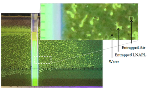
Figure 1. LNAPL Distribution in a research sand tank
[5].
Figure 1 shows a research tank with a well screen in a porous media (sand) containing LNAPL. The LNAPL fluoresces under ultraviolet (UV) light, while water and air do not. The column of yellow fluorescence in the well represents the gauged LNAPL thickness and corresponds to the vertical interval over which LNAPL flows in the formation[6]. The yellow fluorescence to the left of the well represents LNAPL occurring within soil pores. Below the potentiometric surface line, the pores are dominated by water (dark pores) and LNAPL. Above this line LNAPL and water still exist in pores, but the air saturation increases with elevation. The incomplete yellow fluorescence in the formation illustrates how water and LNAPL occupy pores over the mobile interval. This occurs because the mobile LNAPL cannot displace all of the water from the pores.
LNAPL mobility can be described mathematically by Darcy’s Law, an empirically derived equation describing the flow of fluids through porous media where the specific discharge, q, is equal to the product of the hydraulic conductivity, K, and the hydraulic gradient, i. While this is the same Darcy’s Law that is used to describe groundwater flow (see Advection and Groundwater Flow), there is an important additional term, Relative Permeability, that is included when using Darcy’s Law to describe the flow of LNAPL in the subsurface. Relative permeability is the ratio of the effective permeability of a fluid at a specified saturation to the intrinsic permeability of the medium at 100-percent saturation[7]. The USEPA (1996)[8] describes relative permeability this way:
References
- ^ 1.0 1.1 ITRC, 2018. LNAPL Site Management: LCSM evolution, decision process, and remedial technologies (LNAPL-3). Interstate Technical and Regulatory Council
- ^ Charbeneau, R.J., 2007. LNAPL Distribution and Recovery Model. Distribution and Recovery of Petroleum Hydrocarbon Liquids in Porous Media. Vol. 1. API Publication 4760. Report.pdf
- ^ 3.0 3.1 CRC CARE, 2018. Technical measurement guidance for LNAPL natural source zone depletion. Cooperative Research Centre for Contamination Assessment and Remediation of the Environment, Newcastle, Australia. Technical Report no. 44. 254p Report.pdf
- ^ Mahler, N., Sale, T. and Lyverse, M., 2012. A mass balance approach to resolving LNAPL stability. Groundwater, 50(6), pp.861-871. [10.1111/j.1745-6584.2012.00949.x 10.1111/j.1745-6584.2012.00949.x
- ^ Hawkins, A. M., 2013. Processes Controlling the behavior of LNAPLs at groundwater surface water interfaces, Master of Science Thesis, Colorado State University, Ft. Collins, Colorado. Report.pdf
- ^ Huntley, D., 2000. Analytic determination of hydrocarbon transmissivity from baildown tests. Groundwater, 38(1), pp.46-52. doi: 10.1111/j.1745-6584.2000.tb00201.x
- ^ Mercer, J.W. and Cohen, R.M., 1990. A review of immiscible fluids in the subsurface: properties, models, characterization and remediation. Journal of contaminant hydrology, 6(2), pp.107-163. [Mercer, J.W. and Cohen, R.M., 1990. A review of immiscible fluids in the subsurface: properties, models, characterization and remediation. Journal of contaminant hydrology, 6(2), pp.107-163. doi: 10.1016/0169-7722(90)90043-G
- ^ USEPA, 1996. How to effectively recover free product at leaking underground storage sites. A guide for state regulators. USEPA 510-R-96-001. U.S. Environmental Protection Agency, 162 pp. Report.pdf
See Also
