Difference between revisions of "User:Jhurley/sandbox"

Revision as of 19:05, 1 February 2024

Hydrogeophysical methods for characterization and monitoring of surface water-groundwater interactions

Hydrogeophysical methods can be used to cost-effectively locate and characterize regions of enhanced groundwater/surface-water exchange (GWSWE) and to guide effective follow up investigations based on more traditional invasive methods. The most established methods exploit the contrasts in temperature and/or specific conductance that commonly exist between groundwater and surface water.

1 Hydrogeophysical methods for characterization and monitoring of surface water-groundwater interactions
2 Introduction
3 Hydrogeophysical Technologies for Understanding Groundwater-Surface Water Interactions
4 Guidelines for Implementing Hydrogeophysical Methods into Groundwater/Surface Water Interaction Studies
5 Summary
6 References
7 See Also

Related Article(s):

Contributor(s):

Dr. Lee Slater
Dr. Ramona Iery
Dr. Dimitrios Ntarlagiannis
Henry Moore

Key Resource(s):

USGS Method Selection Tool: https://code.usgs.gov/water/espd/hgb/gw-sw-mst
USGS Water Resources: https://www.usgs.gov/mission-areas/water-resources/science/groundwatersurface-water-interaction

Introduction

Discharges of contaminated groundwater to surface water bodies threaten ecosystems and degrade the quality of surface water resources. Subsurface heterogeneity associated with the geological setting and stratigraphy often results in such discharges occurring as localized zones (or seeps) of contaminated groundwater. Traditional methods for investigating GWSWE include seepage meters^[1]^[2], which directly quantify the volume flux crossing the bed of a surface water body (i.e, a lake, river or wetland) and point probes that locally measure key water quality parameters (e.g., temperature, pore water velocity, specific conductance, dissolved oxygen, pH). Seepage meters provide direct estimates of seepage fluxes between groundwater and surface- water but are time consuming and can be difficult to deploy in high energy surface water environments and along armored bed sediments. Manual seepage meters rely on quantifying volume changes in a bag of water that is hydraulically connected to the bed. Although automated seepage meters such as the Ultraseep system have been developed, they are generally not suitable for long term deployment (weeks to months). The US Navy has developed the Trident probe for more rapid (relative to seepage meters) sampling, whereby the probe is inserted into the bed and point-in-time pore water quality and sediment parameters are directly recorded (note that the Trident probe does not measure a seepage flux). Such direct probe-based measurements are still relatively time consuming to acquire, particularly when reconnaissance information is required over large areas to determine the location of discrete seeps for further, more quantitative analysis.

Over the last few decades, a broader toolbox of hydrogeophysical technologies has been developed to rapidly and non-invasively evaluate zones of GWSWE in a variety of surface water settings, spanning from freshwater bodies to saline coastal environments. Many of these technologies are currently being deployed under a Department of Defense Environmental Security Technology Certification Program (ESTCP) project (ER21-5237) to demonstrate the value of the toolbox to remedial program managers (RPMs) dealing with the challenge of characterizing surface water contamination via groundwater from facilities proximal to surface water bodies. This article summarizes these technologies and provides references to key resources, mostly provided by the Water Resources Mission Area of the United States Geological Survey that describe the technologies in further detail.

Hydrogeophysical Technologies for Understanding Groundwater-Surface Water Interactions

Hydrogeophysical technologies exploit contrasts in the physical properties between groundwater and surface water to detect and monitor zones of pronounced GWSWE. The two most valuable properties to measure are temperature and electrical conductivity. Temperature has been used for decades as an indicator of groundwater-surface water exchange^[3] with early uses including pushing a thermistor into the bed of a surface water body to assess zones of surface water downwelling and groundwater upwelling. Today, a variety of novel technologies that measure temperature over a wide range of spatial and temporal scales are being used to investigate GWSWE. The evaluation of electrical conductivity measurements using point probes and geophysical imaging is also well-established. However, new technologies are now available to exploit electrical conductivity contrasts from GWSWE occurring over a range of spatial and temporal scales.

Temperature-Based Technologies

Several temperature-based GWSWE methodologies exploit the gradient in temperature between surface water and groundwater that exist during certain times of day or seasons of the year. The thermal insulation provided by the Earth’s land surface means that groundwater is warmer than surface water in winter months, but colder than surface water in summer months away from the equator. Therefore, in temperate climates, localized (or ‘preferential’) groundwater discharge into surface water bodies is often observed as cold temperature anomalies in the summer and warm temperature anomalies in the winter. However, there are times of the year such as fall and spring when contrasts in the temperature between groundwater and surface water will be minimal, or even undetectable. These seasonal-driven points in time correspond to the switch in the polarity of the temperature contrast between groundwater and surface water. Consequently, SW to GW gradient temperature-based methods are most effective when deployed at times of the year when the temperature contrasts between groundwater and surface water are greatest. Other time-series temperature monitoring methods depend more on natural daily signals measured at the bed interface and in bed sediments, and those signals may exist year round except where strongly muted by ice cover or surface water stratification. A variety of sensing technologies now exist within the GWSWE toolbox, from techniques that rapidly characterize temperature contrasts over large areas, down to powerful monitoring methods that can continuously quantify GWSWE fluxes at discrete locations identified as hotspots.

Characterization Methods

The primary use of the characterization methods is to rapidly determine precise locations of groundwater upwelling over large areas in order to pinpoint locations for subsequent ground-based observations. A common limitation of these methods is that they can only sense groundwater fluxes into surface water. Methods applied at the water surface and in the surface water column generally cannot detect localized regions of surface water transfer to groundwater, for which temperature measurements collected within the bed sediments are needed. This is a more challenging characterization task that may, in the right conditions, be addressed using electrical conductivity-based methods described later in this article.

Unmanned Aerial Vehicle Infrared (UAV-IR)

Figure 1. UAV IR orthomosaics with estimated scale of (a) a wetland in winter (modified from Briggs et al.^[4]) and (b) a mountain stream in summer (modified from Briggs et al.^[5]) that both capture multiscale groundwater discharge processes. Figure reproduced from Mangel et al.^[6]

Unmanned aerial vehicles (UAVs) equipped with thermal infrared (IR) cameras can provide a very powerful tool for rapidly determining zones of pronounced upwelling of groundwater to surface water. Large areas of can be covered with high spatial resolution. The information obtained can be used to rapidly define locations of focused groundwater upwelling and prioritize these for more intensive surface-based observations (Figure 1). As with all thermal methods, flights must be performed when adequate contrasts in temperature between surface water and groundwater are expected to exist. Not just time of year but, because of the effect of the diurnal temperature signal on surface water bodies, time of day might need to be considered in order to maximize the chance of success. Calibration of UAV-IR camera measurements against simultaneously acquired direct measurements of temperature is recommended to optimize the value of these datasets. UAV-IR methods will not work in all situations. One major limitation of the technology is that the temperature expression of groundwater upwelling must be manifested at the surface of the surface water body. Consequently, the technology will not detect relatively small discharges occurring beneath a relatively deep surface water layer, and thermal imaging over the water surface can be complicated by thermal IR reflection. The chances of success with UAV-IR will be strongest in regions of exposed banks or shallow water where there are no strong currents causing mixing (and thus dilution) of the upwelling groundwater temperature signals. UAV-IR methods will therefore likely be most successful close to shorelines of lakes/ponds, over shallow, low flow streams and rivers and in wetland environments. UAV-IR methods require a licensed pilot, and restrictions on the use of airspace may limit the application of this technology.

Handheld Thermal Infrared (TIR) Cameras

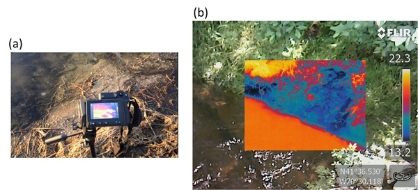
Figure 2. (a) A TIR camera set up to image groundwater discharges to surface water (b) TIR data inset on a visible light photograph. Cooler (blue) bank seepage groundwater is discharging into warmer (red) stream water (temperature scale in degrees). Both photographs courtesy of Martin Briggs USGS.

Hand-held thermal infrared (TIR) cameras are powerful tools for visual identification of localized seeps of upwelling groundwater. TIR cameras may be used to follow up on UAV-IR surveys to better characterize local seeps identified from the air using UAV-IR. Alternatively, a TIR camera is a valuable tool when performing initial walks of prospective study sites as they may quickly confirm the presence of suspected seeps. TIR cameras provide high resolution images that can define the structure of localized seeps and may provide valuable insights into the role of discrete features (e.g., fractures in rocks or pipes in soil) in determining seep morphology (Figure 2). Like UAV-IR, TIR provides primarily qualitative information (location, extent) of seeps and it only succeeds when there are adequate contrasts between groundwater and surface water that are expressed at the surface of the investigated water body or along bank sediments. The United States Geological Survey (USGS) has made extensive use of TIR cameras for studying groundwater/surface-water exchange.

Continuous Near-bed Temperature Sensing

When performing surveys from a boat a simple yet often powerful technology is continuous near-bed temperature sensing, whereby a temperature probe is strategically suspended to float in the water column just above the bed or dragged along it. Compared to UAV-IR, this approach does not rely on upwelling groundwater being expressed as a temperature anomaly at the surface. The utility of the method can be enhanced when a specific conductance probe is co- located with the temperature probe so that anomalies in both temperature and specific conductance can be investigated.

Monitoring Methods

Monitoring methods allow temperature signals to be recorded with high temporal resolution along the bed interface or within bank or bed sediments. These methods can capture temporal trends in GWSWE driven by variations in the hydraulic gradients around surface water bodies, as well as changes in hydraulic conductivity due to sedimentation, clogging, scour or microbial mass. If vertical profiles of bed temperature are collected, a range of analytical and numerical models can be applied to infer the vertical water flux rate and direction, similar to a seepage meter. These fluxes may vary as a function of season, rainfall events (enhanced during storm activity), tidal variability in coastal settings and due to engineered controls such as dam discharges. The methods can capture evidence of GWSWE that may not be detected during a single ‘characterization’ survey if the local hydraulic conditions at that point in time result in relatively weak hydraulic gradients.

Fiber-optic Distributed Temperature Sensing (FO-DTS)

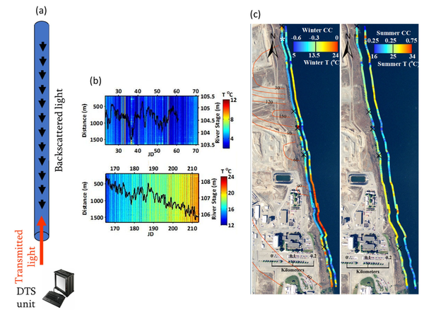
Figure 3. (a) Basic concept of FO-DTS based on backscattering of light transmitted down a FO fiber (b) Example of riverbed temperature data acquired over time and space in relation to variation in river stage (black line) modified from Mwakanyamale et al.^[7] (c) spatial distribution of riverbed temperature and correlation coefficient (CC) between riverbed temperature and river stage for a 1.5 km stretch along the Hanford 300 Area adjacent to the Columbia River (modified from Slater et al.^[8]). Data are shown for winter and summer. Orange contours show uranium concentrations (μg/L) in groundwater measured in boreholes.

Fiber-optic distributed temperature sensing (FO-DTS) is a powerful monitoring technology used in fire detection, industrial process monitoring, and petroleum reservoir monitoring. The method is also used to obtain spatially rich datasets for monitoring GWSWE^[9]^[10]. The sensor consists of standard telecommunications fiber-optic fiber typically housed in armored cable and the physics is based on temperature-dependent backscatter mechanisms including Brillouin and Raman backscatter^[9]. Most commercially available systems are based on analysis of Raman scatter. As laser light is transmitted down the fiber-optic cable, light scatters continuously back toward the instrument from all along the fiber, with some of the scattered light at frequencies above and below the frequency of incident light, i.e., anti-Stokes and Stokes-Raman backscatter, respectively. The ratio of anti-Stokes to Stokes energy provides the basis for FO-DTS measurements. Measurements are localized to a section of cable according to a time-of-flight calculation (i.e., optical time-domain reflectometry). Assuming the speed of light within the fiber is constant, scatter collected over a specific time window corresponds to a specific spatial interval of the fiber. Although there are tradeoffs between spatial resolution, thermal precision, and sampling time, in practice it is possible to achieve sub meter-scale spatial and approximate 0.1°C thermal precision for measurement cycle times on the order of minutes and cables extending several kilometers^[10]; thus, thousands of temperature measurements can be made simultaneously along a single cable. The method allows the visualization of a large amount of temperature data and rapid identification of major trends in GWSWE. Figure 3 illustrates the use of FO-DTS to detect and monitor zones of focused groundwater discharge along a 1.5 km reach of the Columbia River that is threatened by contaminated groundwater^[8]. As temperature is only sensed at the cable on the bed, FO-DTS can only detect groundwater inputs to surface water. It cannot detect losses of surface water to groundwater. The USGS public domain software tool DTSGUI allows a user to import, manage, visualize and analyze FO-DTS datasets.

Vertical temperature profilers (VTPs)

Analysis methods now allow for the accurate quantification of groundwater fluxes over time. Vertical temperature profilers (VTPs) are sensors applied for diurnal temperature data collection within saturated geologic matrices (Figure 4). Extensive experience with VTPs indicates that the methodology is equal to traditional seepage meters in terms of flux accuracy^[11]. However, VTPs have the advantage of measuring continuous temporal variations in flux rates while such information is impractical to obtain with traditional seepage meters.

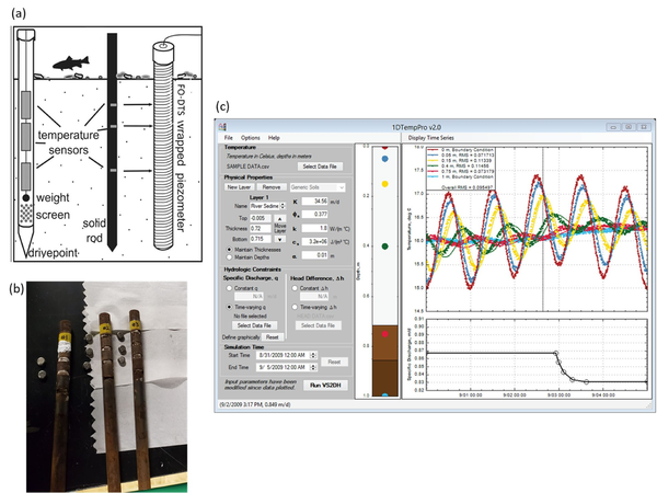
Figure 4. (a) Schematic of different VTP setups including (from left to right) thermistors in a piezometer, thermistors embedded in a solid rod and wrapped FO-DTS cable modified from Irvine et al.^[12]; (b) construction of VTPs showing thermistors embedded in rods and subsequent insulation; (c) example dataset plotted in 1DTempPro showing 5 days of streambed temperature at 6 streambed depths^[13].

The low-cost design, ease of data collection, and straightforward interpretation of the data using open-source software make VTP sensors increasingly attractive for quantifying flux rates. These sensors typically consist of at least two temperature loggers installed within a steel or plastic pipe filled with foam insulation^[12] although the use of loggers installed in well screens or FO-DTS cable wrapped around a piezometer casing (for high vertical resolution data) are also possible (Figure 4a). Loggers are inserted into the insulated housing at different depths, typically starting from one centimeter within the geologic matrix of interest^[14]. Temperature loggers usually remain within the first 0.2-meters of the geologic matrix based on the observed limits of diurnal signal influence^[15], though zones of strong surface water downwelling may necessitate deeper temperature data collection. Reliability of flux values generated from the temperature signal analysis is dependent in part on the temperature logger precision, VTP placement, sediment heterogeneity, flow direction, flow magnitude^[14], and absence of macropore flow. Application of single dimension temperature-based fluid flux models assumes that all flow is vertical and therefore lateral flow within upwelling systems cannot be quantified using VTPs, emphasizing the importance of the VTP installation location over the active area of exchange^[14] at shallow depths. Thermal parameters of the geologic matrix where the VTP is installed can be measured using a thermal properties analyzer to record heat capacity and thermal conductivity for later analytical and numerical modeling.

Analytical and numerical solutions, used to solve or estimate the advection-conduction equation within the geologic matrix (bed sediments), continue to evolve to better quantify flux values over time. Analytical solutions to the heat transport equation are used to solve for flux values between sensor pairs from VTP datasets^[16]^[17]. VFLUX is an open-source MATLAB package that allows the user to solve for flux values from a VTP dataset using a variety of analytical solutions^[16]^[17] based on the vertical propagation of diurnal temperature signals. Other emerging ‘spectral’ methods make use of a wide range of natural temperature signals to estimate vertical flux and bed sediment thermal diffusivity^[18]. VFLUX analytical solutions are limited by subsurface heterogeneity and diurnal temperature signal strength^[14]. 1DTempPro (Figure 4c) provides a graphical user interface (GUI) for numerical solutions to heat transport^[19] and does not depend on diurnal signals. Numerical models can produce more accurate flux estimates in the case of complex boundary conditions and abrupt changes in flux rates, but require significant user calibration efforts for longer time series^[20]. A hybrid approach between the analytical and numerical solutions, known as tempest1d^[20] improves flux modeling with enhanced computational efficiency, resolution of abrupt changes, evaluation of complex boundary conditions, and uncertainty estimations with each step. This new state-space modeling approach uses recursive estimation techniques to automatically estimate highly dynamic vertical flux patterns ranging from sub-daily to seasonal time scales^[20].

Electrical Conductivity (EC) Based Technologies

The electrical conductivity (EC)-based technologies exploit contrasts in EC between surface water and groundwater^[21]. EC-based technologies are mostly applied as characterization tools, although the opportunity to monitor GWSWE dynamics with one of these technologies does exist. With the exception of specific conductance probes, the technologies measure the bulk EC of sediments, which will often (but not always) reveal evidence of GWSWE.

Electrical conduction (i.e., the transport of charges) in the Earth occurs via the ions dissolved in groundwater, with an additional contribution from ions in the electrical double layer (known as surface conduction)^[22]. In relatively fresh surface water environments, groundwater is typically more electrically conductive than surface water due to the higher ion concentrations in groundwater. In these settings, groundwater inputs may be identified as zones of higher bulk EC beneath the bed. In coastal settings where surface water is saline, inputs of relatively fresh groundwater will give rise to zones of lower conductivity. Whereas the temperature-based methods rely on point measurements at the location of the sensor, the EC-based technologies (with the exception of point specific conductance measurements) incorporate inverse modeling to estimate distributions of EC away from the sensors and beneath the bed. Consequently, these technologies may also image losses of surface water to groundwater^[23]. Another advantage is that they may provide information on structural controls on zones of focused GWSWE expressed at the surface. However, interpretation of EC patterns from these technologies is inherently uncertain due to the fact that (with the exception of specific conductance probes) the bulk EC of the sediments is measured. Variations in lithology (e.g., porosity, grain size distribution, which determine the strength of surface conduction) can be misinterpreted as variations in the ionic composition of groundwater.

Characterization Methods

Specific Conductance Probes

The simplest EC-based technology is a specific conductance probe, which measures the specific conductance of water between a small pair of metal plates at the end of the sensor probe. Many commercially available water quality sensors have a specific conductance sensor and a temperature sensor integrated into a single probe (they often also measure other water quality parameters, including pH and dissolved oxygen (DO) content). These are direct sensing measurements with a small footprint (the size of the sensor), so this is usually a time-consuming, inefficient method for detecting GWSWE dynamics. Furthermore, the sampling volume of the measurement is small (on the order of a cubic centimeter or less), so the degree to which the spot measurement is representative of larger-scale hydrological exchanges is often uncertain. However, specific conductance sensor remains popular, especially when integrated with a point temperature sensor, such as the Trident Probe.

Frequency Domain Electromagnetic (EM) Sensing Systems

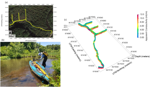
Figure 5. (a) FDEM survey path within a stream/drainage channel network bisecting a wetland complex experiencing localized upwelling of contaminated groundwater (b) operation of an FDEM sensor (Dualem 421S, Dualem, CA) in this shallow stream environment (c) resulting imaging of EC structure in the upper 6 m of streambed sediments. Variations in EC may result from changes in sediment texture that determine the location of focused GWSWE. Dataset acquired under ESTCP project ER21-5237.

Electromagnetic (EM) sensors non-invasively sense the bulk EC of sediments (a function of both fluid composition and lithology as mentioned above) by measuring eddy currents induced in conductors using time varying electric and magnetic fields based on the physics of electromagnetic induction. Modern EM systems can simultaneously image across a range of depths. Frequency domain EM (FDEM) instruments generate a current that varies sinusoidally with time at a fixed frequency that is selected on the basis of desired exploration depth and resolution. State of the art FDEM sensors use a combination of different coil separations and/or frequencies to resolve conductivity structure over a range of depths. These instruments typically provide high-resolution (sub-meter) information on the EC structure in the upper 5 m (approximately, depending on EC) of the subsurface. Measurements are non-invasively and continuously made, meaning that large areas can be quickly surveyed on foot (e.g., along a shoreline) or from a boat in shallow water (1 m or less deep), for example when pulled along a river or stream channel. The method can also be deployed effectively in wetlands (Figure 5). FDEM data are often presented in terms of variations in the raw measurements because apparent EC values do not represent the true EC of the subsurface. However, with the increasing popularity of sensors with combinations of coil separations, the datasets can be inverted to obtain a model of the distribution of the true EC of the subsurface on land or below a water layer. Inversion of FDEM datasets is usually performed as a series of one-dimensional (1D) models, constrained to have a limited variance from each other, to generate a pseudo-2D model of the subsurface. Open-source software, such as EMagPy^[24], is freely available to manage, visualize and interpret FDEM datasets.

Time Domain EM Sensing Systems

Time domain EM (TEM) systems transmit a current that is abruptly shut off (reduced to zero), resulting in a transient current flow that propagates (with decaying amplitude) into the earth. The time-decaying voltage recorded in a receiver coil contains information on the EC variation with depth below the instrument. TEM systems specifically designed for waterborne surveys provide investigation depths up to 70 m (again depending on electrical conductivity)^[25]. Airborne TEM systems can also be deployed to look at large-scale surface water/groundwater dynamics, for example submarine discharge or saline intrusion along coastlines^[26]. Inverse methods are employed to convert the raw measurements obtained along a transect into a distribution of conductivity.

Waterborne Electrical Imaging

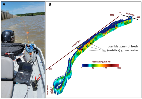
Figure 6. Waterborne electrical imaging in a coastal setting with expected zones of upwelling groundwater (a) typical operation with floating electrode cable pulled behind boat (b) inverted 2D cross section of electrical resistivity along the survey path with possible zones of fresh groundwater discharges indicated from relatively high resistivity sediments. Dataset acquired under ESTCP project ER21-5237.

Electrical imaging techniques are based on galvanic (direct) contact between electrodes used to inject currents (and measure voltages) and the subsurface^[22]. Relative to EM methods, this can be a disadvantage when surveying on land. However, when making measurements from a water body, the electrodes used to acquire the data can be deployed as a floating array that is pulled behind a vessel. Waterborne electrical imaging relies on acquiring measurements of electrical potential differences between different pairs of electrodes on the array while current is passed between one pair of electrodes^[27]. As the array is pulled behind the boat, thousands of measurements are made along a survey transect. Similar to the EM methods, inverse methods are used to process these datasets and generate a 2D image of the variation in the conductivity of the sediments below the bed. Open-source software such as ResIPy support 2D or 3D inversion of waterborne datasets. Figure 6 shows results of a waterborne electrical imaging survey conducted to locate regions where relative fresh (electrically resistive) groundwater is discharging into the near shore environment in a coastal setting. Beneath the saline (low resistivity) water layer, spatial variability in resistivity may partly be related to variations in the pore-filling fluid conductivity, with localized resistive zones possibly indicating upwelling fresh groundwater. However, the variation in resistivity in the sediments below the water layer may reflect variations in lithology. An extension of the electrical imaging method involves collecting induced polarization (IP) data^[22] in addition to electrical resistivity data. IP measurements capture the temporary charge storage characteristics of the subsurface, which are strongly controlled by lithology, with finer-grained (e.g. clay rich) sediments being more chargeable than coarser grained sediments. The method can be particularly useful for differentiating between conductivity variations resulting from variations in pore fluid specific conductance and those conductivity variations associated with lithology. For example, based on electrical imaging methods alone (or the EM method alone), it may not be possible to distinguish a zone of high specific conductance groundwater entering into freshwater from a region of relatively finer- grained sediments without additional supporting data (e.g. a core). IP measurements may be able to resolve this ambiguity as the region of finer-grained sediments will be more chargeable than the surrounding areas.

Monitoring Methods

Land-based Electrical Monitoring

There is increasing interest in the use of electrical imaging methods as monitoring systems. Semi-permanent arrays of electrodes can be installed to monitor groundwater/surface water dynamics over periods of days to years. Low-power instrumentation has been developed to specifically address the needs for long-term monitoring, although such instrumentation is not yet commercially available. Consequently, electrical monitoring of groundwater/surface water interactions currently remains in the realm of the research-driven specialist.

Considerations for Using EM and Waterborne Electrical Imaging Methods

The EM and waterborne electrical imaging methods both provide a way to determine variations in bulk electrical conductivity associated with groundwater/surface water interactions. However, each method has some advantages and some disadvantages. One consideration is maneuverability, particularly in shallow water environments. FDEM instruments are the most maneuverable, although they offer only limited investigation depths. Although bigger than the shallow-sensing frequency domain EM systems, TEM systems are still relatively maneuverable on water bodies. Whereas FDEM systems can be operated from a single small vessel, the TEM deployments require the use of pontoons as the transmitter and receiver coils need to be separated 9 m apart. This still equates to good maneuverability compared to waterborne electrical imaging where a floating electrode cable, typically 30-50 m long, is pulled behind a vessel.

In all three methods, variations in the water layer depth and the specific conductance of the water can significantly affect the data, especially in deeper water. Therefore, it is common to continuously record these parameters with an echo sounder and a specific conductance probe suspended in the water layer.

Other Hydrogeophysical Technologies

A number of other hydrogeophysical technologies exist, with proven applications to the characterization of settings where GWSWE occurs. Seismic reflection and refraction methods are used to image the depositional environments along coastlines. Ground penetrating radar has been effectively used to image depositional environments around freshwater lake shorelines, and across streams and rivers. Such information may help to identify depositional features that promote GWSWE but, unlike the temperature- and conductivity-based methods, do not sense changes in physical properties associated with the exchanging water itself.

One promising technique for detecting GWSWE is known as the self-potential (SP) method. This simple to deploy geophysical technique is based on mapping voltage differences caused by natural sources of electric current in the Earth that are generated through a number of coupled flow processes, one being the coupling of pore fluid flow and transport of electric charge. Zones of enhanced seepage within a porous medium can result in a significant ‘streaming potential’ due to charge transport induced by fluid flow. This phenomenon has been effectively used to locate zones of leakage through dams and embankments^[28]. Recently, floating SP measurements have been used to define gaining and losing portions of streams and to identify evidence of focused exchange^[29]. Although the data acquisition is simple, consisting of a pair of non-polarizing electrodes and a voltmeter, the interpretation of SP measurements requires expert knowledge to filter out confounding contributions to the recorded signals.

Guidelines for Implementing Hydrogeophysical Methods into Groundwater/Surface Water Interaction Studies

A number of factors will affect the success of individual hydrogeophysical methods at a specific site of GWSWE. Depending on site conditions and the objective, some methods may be inappropriate to deploy. For example, temperature-based methods will most likely succeed at times of the year and times of day when contrasts between upwelling groundwater and surface water are greatest. In contrast, it is quite possible that some sites of groundwater/surface water exchange will have an insufficient contrast in the specific conductance of the groundwater versus the surface water to make techniques based on EC measurements effective. A groundwater-surface water method selection tool (GW/SW-MST^[30]) has recently been developed to assist practitioners in the informed selection of the methods that will be most effective for a particular site at a particular time. The tool guides the user through a series of questions that consider both the specific conditions at the site and the primary objectives of the investigation. The methods selection tool discusses the application of a number of additional technologies besides those included in this article. The selection tool is recommended as the starting point for any practitioner.

Summary

A number of temperature-based and electrical conductivity-based technologies exist for monitoring GWSWE over a range of spatial scales. Many of these technologies are most powerful when used as reconnaissance tools to rapidly identify probable locations of GWSWE to be verified with a limited campaign of direct sensing measurements (traditionally seepage meters). Vertical temperature profilers (VTPs) offer direct quantification of fluxes at sites identified by the reconnaissance tools, and some studies show that these methods are more reliable than traditional seepage meters. Given the number of sites across the globe where contaminated groundwater is impacting surface water resources, use of these technologies for both characterization and monitoring is expected to become more common.

References

^ Rosenberry, D. O., Duque, C., and Lee, D. R., 2020. History and Evolution of Seepage Meters for Quantifying Flow between Groundwater and Surface Water: Part 1 – Freshwater Settings. Earth-Science Reviews, 204(103167). doi: 10.1016/j.earscirev.2020.103167.
^ Duque, C., Russoniello, C. J., and Rosenberry, D. O., 2020. History and Evolution of Seepage Meters for Quantifying Flow between Groundwater and Surface Water: Part 2 – Marine Settings and Submarine Groundwater Discharge. Earth-Science Reviews, 204 ( 103168). doi: 10.1016/j.earscirev.2020.103168.
^ Constantz, J., 2008. Heat as a Tracer to Determine Streambed Water Exchanges. Water Resources Research, 44 (4).doi: 10.1029/2008WR006996.Open Access Article
^ Briggs, M. A., Jackson, K. E., Liu, F., Moore, E. M., Bisson, A., Helton, A. M., 2022. Exploring Local Riverbank Sediment Controls on the Occurrence of Preferential Groundwater Discharge Points. Water, 14(1). doi: 10.3390/w14010011 Open Access Article.
^ Briggs, M. A., Wang, C., Day-Lewis, F. D., Williams, K. H., Dong, W., Lane, J. W., 2019. Return Flows from Beaver Ponds Enhance Floodplain-to-River Metals Exchange in Alluvial Mountain Catchments. Science of the Total Environment, 685, pp. 357–369. doi: 10.1016/j.scitotenv.2019.05.371. Open Access Manuscript
^ Mangel, A. R., Dawson, C. B., Rey, D. M., Briggs, M. A., 2022. Drone Applications in Hydrogeophysics: Recent Examples and a Vision for the Future. The Leading Edge, 41 (8), pp. 540–547. doi: 10.1190/tle41080540.
^ Mwakanyamale, K., Slater, L., Day-Lewis, F., Elwaseif, M., Johnson, C., 2012. Spatially Variable Stage-Driven Groundwater-Surface Water Interaction Inferred from Time-Frequency Analysis of Distributed Temperature Sensing Data. Geophysical Research Letters, 39(6). doi: 10.1029/2011GL050824. Open Access Article
^ ^8.0 ^8.1 Slater, L. D., Ntarlagiannis, D., Day-Lewis, F. D., Mwakanyamale, K., Versteeg, R. J., Ward, A., Strickland, C., Johnson, C. D., Lane Jr., J. W., 2010. Use of Electrical Imaging and Distributed Temperature Sensing Methods to Characterize Surface Water-Groundwater Exchange Regulating Uranium Transport at the Hanford 300 Area, Washington. Water Resources Research, 46(10). doi: 10.1029/2010WR009110. Open Access Article
^ ^9.0 ^9.1 Selker, J. S., Thévenaz, L., Huwald, H., Mallet, A., Luxemburg, W., van de Giesen, N., Stejskal, M., Zeman, J., Westhoff, M., Parlange, M. B., 2006. Distributed Fiber-Optic Temperature Sensing for Hydrologic Systems. Water Resources Research, 42 (12). doi: 10.1029/2006WR005326. Open Access Article
^ ^10.0 ^10.1 Tyler, S. W., Selker, J. S., Hausner, M. B., Hatch, C. E., Torgersen, T., Thodal, C. E., Schladow, S. G., 2009. Environmental Temperature Sensing Using Raman Spectra DTS Fiber-Optic Methods. Water Resources Research, 45(4). doi: 10.1029/2008WR007052. Open Access Article
^ Hare, D. K., Briggs, M. A., Rosenberry, D. O., Boutt, D. F., Lane Jr., J. W., 2015. A Comparison of Thermal Infrared to Fiber-Optic Distributed Temperature Sensing for Evaluation of Groundwater Discharge to Surface Water. Journal of Hydrology, 530, pp. 153–166. doi: 10.1016/j.jhydrol.2015.09.059.
^ ^12.0 ^12.1 Irvine, D. J., Briggs, M. A., Cartwright, I., Scruggs, C. R., Lautz, L. K., 2016. Improved Vertical Streambed Flux Estimation Using Multiple Diurnal Temperature Methods in Series. Groundwater, 55(1), pp. 73-80. doi: 10.1111/gwat.12436.
^ Koch, F. W., Voytek, E. B., Day-Lewis, F. D., Healy, R., Briggs, M. A., Lane Jr., J. W., Werkema, D., 2016. 1DTempPro V2: New Features for Inferring Groundwater/Surface-Water Exchange. Groundwater, 54(3), pp. 434–439. doi: 10.1111/gwat.12369.
^ ^14.0 ^14.1 ^14.2 ^14.3 Irvine, D. J., Briggs, M. A., Lautz, L. K., Gordon, R. P., McKenzie, J. M., Cartwright, I., 2017. Using Diurnal Temperature Signals to Infer Vertical Groundwater-Surface Water Exchange. Groundwater, 55(1), pp. 10–26. doi: 10.1111/gwat.12459. Open Access Manuscript
^ Briggs, M. A., Lautz, L. K., Buckley, S. F., Lane Jr., J. W., 2014. Practical Limitations on the Use of Diurnal Temperature Signals to Quantify Groundwater Upwelling. Journal of Hydrology, 519(B), pp. 1739–1751. doi: 10.1016/j.jhydrol.2014.09.030.
^ ^16.0 ^16.1 Gordon, R. P., Lautz, L. K., Briggs, M. A., McKenzie, J. M., 2012. Automated Calculation of Vertical Pore-Water Flux from Field Temperature Time Series Using the VFLUX Method and Computer Program. Journal of Hydrology, 420–421, pp. 142–158. doi: 10.1016/j.jhydrol.2011.11.053.
^ ^17.0 ^17.1 Irvine, D. J., Lautz, L. K., Briggs, M. A., Gordon, R. P., McKenzie, J. M., 2015. Experimental Evaluation of the Applicability of Phase, Amplitude, and Combined Methods to Determine Water Flux and Thermal Diffusivity from Temperature Time Series Using VFLUX 2. Journal of Hydrology, 531(3), pp. 728–737. doi: 10.1016/j.jhydrol.2015.10.054.
^ Sohn, R. A., Harris, R. N., 2021. Spectral Analysis of Vertical Temperature Profile Time-Series Data in Yellowstone Lake Sediments. Water Resources Research, 57(4), e2020WR028430. doi: 10.1029/2020WR028430. Open Access Article
^ Koch, F. W., Voytek, E. B., Day-Lewis, F. D., Healy, R., Briggs, M. A., Werkema, D., Lane Jr., J. W., 2015. 1DTempPro: A Program for Analysis of Vertical One-Dimensional (1D) Temperature Profiles v2.0. U.S. Geological Survey Software Release. doi: 10.5066/F76T0JQS. Free Download from USGS
^ ^20.0 ^20.1 ^20.2 McAliley, W. A., Day-Lewis, F. D., Rey, D., Briggs, M. A., Shapiro, A. M., Werkema, D., 2022. Application of Recursive Estimation to Heat Tracing for Groundwater/Surface-Water Exchange. Water Resources Research, 58(6), e2021WR030443. doi: 10.1029/2021WR030443. Open Access Article
^ Cox, M. H., Su, G. W., Constantz, J., 2007. Heat, Chloride, and Specific Conductance as Ground Water Tracers near Streams. Groundwater, 45(2), pp. 187–195. doi: 10.1111/j.1745-6584.2006.00276.x.
^ ^22.0 ^22.1 ^22.2 Binley, A., Slater, L., 2020. Resistivity and Induced Polarization: Theory and Applications to the Near-Surface Earth. Cambridge University Press. doi: 10.1017/9781108685955.
^ Johnson, T. C., Slater, L. D., Ntarlagiannis, D., Day-Lewis, F. D., Elwaseif, M., 2012. Monitoring Groundwater-Surface Water Interaction Using Time-Series and Time- Frequency Analysis of Transient Three-Dimensional Electrical Resistivity Changes. Water Resources Research, 48(7). doi: 10.1029/2012WR011893. Open Access Article
^ McLachlan, P., Blanchy, G., Binley, A., 2021. EMagPy: Open-Source Standalone Software for Processing, Forward Modeling and Inversion of Electromagnetic Induction Data. Computers and Geosciences, 146, 104561. doi: 10.1016/j.cageo.2020.104561.
^ Lane Jr., J. W., Briggs, M. A., Maurya, P. K., White, E. A., Pedersen, J. B., Auken, E., Terry, N., Minsley, B., Kress, W., LeBlanc, D. R., Adams, R., Johnson, C. D., 2020. Characterizing the Diverse Hydrogeology Underlying Rivers and Estuaries Using New Floating Transient Electromagnetic Methodology. Science of the Total Environment, 740, 140074. doi: 10.1016/j.scitotenv.2020.140074. Open Access Manuscript
^ d’Ozouville, N., Auken, E., Sorensen, K., Violette, S., de Marsily, G., Deffontaines, B., Merlen, G., 2008. Extensive Perched Aquifer and Structural Implications Revealed by 3D Resistivity Mapping in a Galapagos Volcano. Earth and Planetary Science Letters, 269(3–4), pp. 518–522. doi: 10.1016/j.epsl.2008.03.011.
^ Day-Lewis, F. D., White, E. A., Johnson, C. D., Lane Jr, J. W., Belaval, M., 2006. Continuous Resistivity Profiling to Delineate Submarine Groundwater Discharge—Examples and Limitations. The Leading Edge, 25(6), pp. 724–728. doi: 10.1190/1.2210056
^ Panthulu, T. V, Krishnaiah, C., Shirke, J. M., 2001. Detection of Seepage Paths in Earth Dams Using Self-Potential and Electrical Resistivity Methods. Engineering Geology, 59(3-4), pp. 281–295. doi: 10.1016/S0013-7952(00)00082-X.
^ Ikard, S. J., Teeple, A. P., Payne, J. D., Stanton, G. P., Banta, J. R., 2018. New Insights On Scale-Dependent Surface-Groundwater Exchange from a Floating Self-Potential Dipole. Journal of Environmental and Engineering Geophysics, 23(2), pp. 261–287. doi: 10.2113/JEEG23.2.261.
^ Hammett, S., Day-Lewis, F. D., Trottier, B., Barlow, P. M., Briggs, M. A., Delin, G., Harvey, J. W., Johnson, C. D., Lane jr., J. W., Rosenberry, D. O., Werkema, D. D., 2022. GW/SW-MST: A Groundwater/Surface-Water Method Selection Tool. Groundwater, 60(6), pp. 784-791. doi: 10.1111/gwat.13194. Open Access Manuscript

Difference between revisions of "User:Jhurley/sandbox"

Revision as of 19:05, 1 February 2024

Hydrogeophysical methods for characterization and monitoring of surface water-groundwater interactions

Contents

Introduction

Hydrogeophysical Technologies for Understanding Groundwater-Surface Water Interactions

Temperature-Based Technologies

Characterization Methods

Unmanned Aerial Vehicle Infrared (UAV-IR)

Handheld Thermal Infrared (TIR) Cameras

Continuous Near-bed Temperature Sensing

Monitoring Methods

Fiber-optic Distributed Temperature Sensing (FO-DTS)

Vertical temperature profilers (VTPs)

Electrical Conductivity (EC) Based Technologies

Characterization Methods

Specific Conductance Probes

Frequency Domain Electromagnetic (EM) Sensing Systems

Time Domain EM Sensing Systems

Waterborne Electrical Imaging

Monitoring Methods

Land-based Electrical Monitoring

Considerations for Using EM and Waterborne Electrical Imaging Methods

Other Hydrogeophysical Technologies

Guidelines for Implementing Hydrogeophysical Methods into Groundwater/Surface Water Interaction Studies

Summary

References

See Also

Navigation menu

Personal tools

Namespaces

Variants

Views

More

Search

Navigation

Topic Categories

Tools

Admin Tools

@@ Line 96: / Line 96: @@
 One promising technique for detecting GWSWE is known as the [https://www.epa.gov/environmental-geophysics/self-potential-sp self-potential (SP)] method. This simple to deploy geophysical technique is based on mapping voltage differences caused by natural sources of electric current in the Earth that are generated through a number of coupled flow processes, one being the coupling of pore fluid flow and transport of electric charge. Zones of enhanced seepage within a porous medium can result in a significant ‘streaming potential’ due to charge transport induced by fluid flow. This phenomenon has been effectively used to locate zones of leakage through dams and embankments<ref>Panthulu, T. V, Krishnaiah, C., Shirke, J. M., 2001. Detection of Seepage Paths in Earth Dams Using Self-Potential and Electrical Resistivity Methods. Engineering Geology, 59(3-4), pp. 281–295. [https://doi.org/10.1016/S0013-7952(00)00082-X doi: 10.1016/S0013-7952(00)00082-X].</ref>. Recently, floating SP measurements have been used to define gaining and losing portions of streams and to identify evidence of focused exchange<ref>Ikard, S. J., Teeple, A. P., Payne, J. D., Stanton, G. P., Banta, J. R., 2018. New Insights On Scale-Dependent Surface-Groundwater Exchange from a Floating Self-Potential Dipole. Journal of Environmental and Engineering Geophysics, 23(2), pp. 261–287. [https://doi.org/10.2113/JEEG23.2.261 doi: 10.2113/JEEG23.2.261].</ref>. Although the data acquisition is simple, consisting of a pair of non-polarizing electrodes and a voltmeter, the interpretation of SP measurements requires expert knowledge to filter out confounding contributions to the recorded signals.
+==Guidelines for Implementing Hydrogeophysical Methods into Groundwater/Surface Water Interaction Studies==
+A number of factors will affect the success of individual hydrogeophysical methods at a specific
+site of GWSWE. Depending on site conditions and the objective, some methods may be inappropriate to deploy. For example, temperature-based methods will most likely succeed at times of the year and times of day when contrasts between upwelling groundwater and surface water are greatest. In contrast, it is quite possible that some sites of groundwater/surface water exchange will have an insufficient contrast in the specific conductance of the groundwater versus the surface water to make techniques based on EC measurements effective. A groundwater-surface water method selection tool ([https://water.usgs.gov/water-resources/software/GW-SW-MST/ GW/SW-MST]<ref>Hammett, S., Day-Lewis, F. D., Trottier, B., Barlow, P. M., Briggs, M. A., Delin, G., Harvey, J. W., Johnson, C. D., Lane jr., J. W., Rosenberry, D. O., Werkema, D. D., 2022. GW/SW-MST: A Groundwater/Surface-Water Method Selection Tool. Groundwater, 60(6), pp. 784-791. [https://doi.org/10.1111/gwat.13194 doi: 10.1111/gwat.13194].&nbsp;&nbsp;[https://ngwa.onlinelibrary.wiley.com/doi/am-pdf/10.1111/gwat.13194 Open Access Manuscript]</ref>) has recently been developed to assist practitioners in the informed selection of the methods that will be most effective for a particular site at a particular time. The tool guides the user through a series of questions that consider both the specific conditions at the site and the primary objectives of the investigation. The methods selection tool discusses the application of a number of additional technologies besides those included in this article. The selection tool is recommended as the starting point for any practitioner.
+==Summary==
+A number of temperature-based and electrical conductivity-based technologies exist for monitoring GWSWE over a range of spatial scales. Many of these technologies are most powerful when used as reconnaissance tools to rapidly identify probable locations of GWSWE to be verified with a limited campaign of direct sensing measurements (traditionally seepage meters). Vertical temperature profilers (VTPs) offer direct quantification of fluxes at sites identified by the reconnaissance tools, and some studies show that these methods are more reliable than traditional seepage meters. Given the number of sites across the globe where contaminated groundwater is impacting surface water resources, use of these technologies for both characterization and monitoring is expected to become more common.
-Hydroquinones have been widely used as surrogates to understand the reductive transformation of NACs and MCs by NOM. Figure 4 shows the chemical structures of the singly deprotonated forms of four hydroquinone species previously used to study NAC/MC reduction. The second-order rate constants (''k<sub>R</sub>'') for the reduction of NACs/MCs by these hydroquinone species are listed in Table 1, along with the aqueous-phase one electron reduction potentials of the NACs/MCs (''E<sub>H</sub><sup>1’</sup>'') where available. ''E<sub>H</sub><sup>1’</sup>'' is an experimentally measurable thermodynamic property that reflects the propensity of a given NAC/MC to accept an electron in water (''E<sub>H</sub><sup>1</sup>''(R-NO<sub>2</sub>)):
-:::::<big>'''Equation 1:'''&nbsp;&nbsp;&nbsp;&nbsp;&nbsp;&nbsp;&nbsp;&nbsp;&nbsp;&nbsp;&nbsp;&nbsp;&nbsp;&nbsp;&nbsp;&nbsp;''R-NO<sub>2</sub> + e<sup>-</sup> ⇔ R-NO<sub>2</sub><sup>•-</sup>''</big>
-Knowing the identity of and reaction order in the reductant is required to derive the second-order rate constants listed in Table 1. This same reason limits the utility of reduction rate constants measured with complex carbonaceous reductants such as NOM<ref name="Dunnivant1992"/>, BC<ref name="Oh2013"/><ref name="Oh2009"/><ref name="Xu2015"/><ref name="Xin2021">Xin, D., 2021. Understanding the Electron Storage Capacity of Pyrogenic Black Carbon: Origin, Redox Reversibility, Spatial Distribution, and Environmental Applications. Doctoral Thesis, University of Delaware.  [https://udspace.udel.edu/bitstream/handle/19716/30105/Xin_udel_0060D_14728.pdf?sequence=1 Free download.]</ref>, and HS<ref name="Luan2010"/><ref name="Murillo-Gelvez2021"/>, whose chemical structures and redox moieties responsible for the reduction, as well as their abundance, are not clearly defined or known. In other words, the observed rate constants in those studies are specific to the experimental conditions (e.g., pH and NOM source and concentration), and may not be easily comparable to other studies.
-{| class="wikitable mw-collapsible" style="float:left; margin-right:40px; text-align:center;"
-|+ Table&nbsp;1.&nbsp;Aqueous&nbsp;phase one electron reduction potentials and logarithm of second-order rate constants for the reduction of NACs and MCs by the singly deprotonated form of the hydroquinones lawsone, juglone, AHQDS and AHQS, with the second-order rate constants for the deprotonated NAC/MC species (i.e., nitrophenolates and NTO<sup>–</sup>) in parentheses.
-|-
-! Compound
-! rowspan="2" |''E<sub>H</sub><sup>1'</sup>'' (V)
-! colspan="4"| Hydroquinone [log ''k<sub>R</sub>''&nbsp;(M<sup>-1</sup>s<sup>-1</sup>)]
-|-
-! (NAC/MC)
-! LAW<sup>-</sup>
-! JUG<sup>-</sup>
-! AHQDS<sup>-</sup>
-! AHQS<sup>-</sup>
-|-
-| Nitrobenzene (NB) || -0.485<ref name="Schwarzenbach1990"/> || 0.380<ref name="Schwarzenbach1990"/> || -1.102<ref name="Schwarzenbach1990"/> || 2.050<ref name="Murillo-Gelvez2019"/> || 3.060<ref name="Murillo-Gelvez2019"/>
-|-
-| 2-nitrotoluene (2-NT) || -0.590<ref name="Schwarzenbach1990"/> || -1.432<ref name="Schwarzenbach1990"/> || -2.523<ref name="Schwarzenbach1990"/> || 0.775<ref name="Hartenbach2008"/> ||
-|-
-| 3-nitrotoluene (3-NT) || -0.475<ref name="Schwarzenbach1990"/> || 0.462<ref name="Schwarzenbach1990"/> || -0.921<ref name="Schwarzenbach1990"/> ||  ||
-|-
-| 4-nitrotoluene (4-NT) || -0.500<ref name="Schwarzenbach1990"/> || 0.041<ref name="Schwarzenbach1990"/> || -1.292<ref name="Schwarzenbach1990"/> || 1.822<ref name="Hartenbach2008"/> || 2.610<ref name="Murillo-Gelvez2019"/>
-|-
-| 2-chloronitrobenzene (2-ClNB) || -0.485<ref name="Schwarzenbach1990"/> || 0.342<ref name="Schwarzenbach1990"/> || -0.824<ref name="Schwarzenbach1990"/> ||2.412<ref name="Hartenbach2008"/> ||
-|-
-| 3-chloronitrobenzene (3-ClNB)	|| -0.405<ref name="Schwarzenbach1990"/> || 1.491<ref name="Schwarzenbach1990"/> || 0.114<ref name="Schwarzenbach1990"/> || ||
-|-
-| 4-chloronitrobenzene (4-ClNB)	|| -0.450<ref name="Schwarzenbach1990"/> || 1.041<ref name="Schwarzenbach1990"/> || -0.301<ref name="Schwarzenbach1990"/> || 2.988<ref name="Hartenbach2008"/> ||
-|-
-| 2-acetylnitrobenzene (2-AcNB)	|| -0.470<ref name="Schwarzenbach1990"/> || 0.519<ref name="Schwarzenbach1990"/> || -0.456<ref name="Schwarzenbach1990"/> || ||
-|-
-| 3-acetylnitrobenzene (3-AcNB)	|| -0.405<ref name="Schwarzenbach1990"/> || 1.663<ref name="Schwarzenbach1990"/> || 0.398<ref name="Schwarzenbach1990"/> || ||
-|-
-| 4-acetylnitrobenzene (4-AcNB)	|| -0.360<ref name="Schwarzenbach1990"/> || 2.519<ref name="Schwarzenbach1990"/> || 1.477<ref name="Schwarzenbach1990"/> || ||
-|-
-| 2-nitrophenol (2-NP) || || 0.568 (0.079)<ref name="Schwarzenbach1990"/> || || ||
-|-
-| 4-nitrophenol (4-NP) || || -0.699 (-1.301)<ref name="Schwarzenbach1990"/> || || ||
-|-
-| 4-methyl-2-nitrophenol (4-Me-2-NP) || || 0.748 (0.176)<ref name="Schwarzenbach1990"/> || || ||
-|-
-| 4-chloro-2-nitrophenol (4-Cl-2-NP) || || 1.602 (1.114)<ref name="Schwarzenbach1990"/> || || ||
-|-
-| 5-fluoro-2-nitrophenol (5-Cl-2-NP) || || 0.447 (-0.155)<ref name="Schwarzenbach1990"/> || || ||
-|-
-| 2,4,6-trinitrotoluene (TNT) || -0.280<ref name="Schwarzenbach2016"/> || || 2.869<ref name="Hofstetter1999"/> || 5.204<ref name="Hartenbach2008"/> ||
-|-
-| 2-amino-4,6-dinitrotoluene (2-A-4,6-DNT) || -0.400<ref name="Schwarzenbach2016"/> || || 0.987<ref name="Hofstetter1999"/> || ||
-|-
-| 4-amino-2,6-dinitrotoluene (4-A-2,6-DNT) || -0.440<ref name="Schwarzenbach2016"/>  || || 0.079<ref name="Hofstetter1999"/> || ||
-|-
-| 2,4-diamino-6-nitrotoluene (2,4-DA-6-NT) || -0.505<ref name="Schwarzenbach2016"/> || || -1.678<ref name="Hofstetter1999"/> || ||
-|-
-| 2,6-diamino-4-nitrotoluene (2,6-DA-4-NT) || -0.495<ref name="Schwarzenbach2016"/> || || -1.252<ref name="Hofstetter1999"/> || ||
-|-
-| 1,3-dinitrobenzene (1,3-DNB) || -0.345<ref name="Hofstetter1999"/> || || 1.785<ref name="Hofstetter1999"/> || ||
-|-
-| 1,4-dinitrobenzene (1,4-DNB) || -0.257<ref name="Hofstetter1999"/> || || 3.839<ref name="Hofstetter1999"/> || ||
-|-
-| 2-nitroaniline (2-NANE) || < -0.560<ref name="Hofstetter1999"/> || || -2.638<ref name="Hofstetter1999"/> || ||
-|-
-| 3-nitroaniline (3-NANE) || -0.500<ref name="Hofstetter1999"/> || || -1.367<ref name="Hofstetter1999"/> || ||
-|-
-| 1,2-dinitrobenzene (1,2-DNB) || -0.290<ref name="Hofstetter1999"/> || || || 5.407<ref name="Hartenbach2008"/> ||
-|-
-| 4-nitroanisole (4-NAN) || || -0.661<ref name="Murillo-Gelvez2019"/> || || 1.220<ref name="Murillo-Gelvez2019"/> ||
-|-
-| 2-amino-4-nitroanisole (2-A-4-NAN) || || -0.924<ref name="Murillo-Gelvez2019"/> || || 1.150<ref name="Murillo-Gelvez2019"/> || 2.190<ref name="Murillo-Gelvez2019"/>
-|-
-| 4-amino-2-nitroanisole (4-A-2-NAN) || || || ||1.610<ref name="Murillo-Gelvez2019"/> || 2.360<ref name="Murillo-Gelvez2019"/>
-|-
-| 2-chloro-4-nitroaniline (2-Cl-5-NANE) || || -0.863<ref name="Murillo-Gelvez2019"/> || || 1.250<ref name="Murillo-Gelvez2019"/> || 2.210<ref name="Murillo-Gelvez2019"/>
-|-
-| N-methyl-4-nitroaniline (MNA) || || -1.740<ref name="Murillo-Gelvez2019"/> || || -0.260<ref name="Murillo-Gelvez2019"/> || 0.692<ref name="Murillo-Gelvez2019"/>
-|-
-| 3-nitro-1,2,4-triazol-5-one (NTO) || || || || 5.701 (1.914)<ref name="Murillo-Gelvez2021"/> ||
-|-
-| Hexahydro-1,3,5-trinitro-1,3,5-triazine (RDX) || || || || -0.349<ref name="Kwon2008"/> ||
-|}
-[[File:AbioMCredFig5.png | thumb |500px|Figure 5. Relative reduction rate constants of the NACs/MCs listed in Table 1 for AHQDS<sup>–</sup>. Rate constants are compared with respect to RDX. Abbreviations of NACs/MCs as listed in Table 1.]]
-Most of the current knowledge about MC degradation is derived from studies using NACs. The reduction kinetics of only four MCs, namely TNT, N-methyl-4-nitroaniline (MNA), NTO, and RDX, have been investigated with hydroquinones. Of these four MCs, only the reduction rates of MNA and TNT have been modeled<ref name="Hofstetter1999"/><ref name="Murillo-Gelvez2019"/><ref name="Riefler2000">Riefler, R.G., and Smets, B.F., 2000. Enzymatic Reduction of 2,4,6-Trinitrotoluene and Related Nitroarenes: Kinetics Linked to One-Electron Redox Potentials. Environmental Science and Technology, 34(18), pp. 3900–3906.  [https://doi.org/10.1021/es991422f DOI: 10.1021/es991422f]</ref><ref name="Salter-Blanc2015">Salter-Blanc, A.J., Bylaska, E.J., Johnston, H.J., and Tratnyek, P.G., 2015. Predicting Reduction Rates of Energetic Nitroaromatic Compounds Using Calculated One-Electron Reduction Potentials. Environmental Science and Technology, 49(6), pp. 3778–3786.  [https://doi.org/10.1021/es505092s DOI: 10.1021/es505092s]&nbsp;&nbsp; [https://pubs.acs.org/doi/pdf/10.1021/es505092s Open access article.]</ref>.
-Using the rate constants obtained with AHQDS<sup>–</sup>, a relative reactivity trend can be obtained (Figure 5). RDX is the slowest reacting MC in Table 1, hence it was selected to calculate the relative rates of reaction (i.e., log ''k<sub>NAC/MC</sub>'' – log ''k<sub>RDX</sub>''). If only the MCs in Figure 5 are considered, the reactivity spans 6 orders of magnitude following the trend: RDX ≈ MNA < NTO<sup>–</sup> < DNAN < TNT < NTO. The rate constant for DNAN reduction by AHQDS<sup>–</sup> is not yet published and hence not included in Table 1. Note that speciation of NACs/MCs can significantly affect their reduction rates. Upon deprotonation, the NAC/MC becomes negatively charged and less reactive as an oxidant (i.e., less prone to accept an electron). As a result, the second-order rate constant can decrease by 0.5-0.6 log unit in the case of nitrophenols and approximately 4 log units in the case of NTO (numbers in parentheses in Table 1)<ref name="Schwarzenbach1990"/><ref name="Murillo-Gelvez2021"/>.
-==Ferruginous Reductants==
-{| class="wikitable mw-collapsible" style="float:right; margin-left:40px; text-align:center;"
-|+ Table&nbsp;2.&nbsp;Logarithm&nbsp;of&nbsp;second-order rate constants for reduction of NACs and MCs by dissolved Fe(II) complexes with the stoichiometry of ligand and iron in square brackets
-|-
-! rowspan="2" | Compound
-! rowspan="2" | E<sub>H</sub><sup>1'</sup>  (V)
-! Cysteine<ref name="Naka2008"/></br>[FeL<sub>2</sub>]<sup>2-</sup>
-! Thioglycolic acid<ref name="Naka2008"/></br>[FeL<sub>2</sub>]<sup>2-</sup>
-! DFOB<ref name="Kim2009"/></br>[FeHL]<sup>0</sup>
-! AcHA<ref name="Kim2009"/></br>[FeL<sub>3</sub>]<sup>-</sup>
-! Tiron <sup>a</sup></br>[FeL<sub>2</sub>]<sup>6-</sup>
-! Fe-Porphyrin <sup>b</sup>
-|-
-! colspan="6" | Fe(II)-Ligand [log ''k<sub>R</sub>'' (M<sup>-1</sup>s<sup>-1</sup>)]
-|-
-| Nitrobenzene || -0.485<ref name="Schwarzenbach1990"/> ||	-0.347	|| 0.874 || 2.235 || -0.136 || 1.424<ref name="Gao2021">Gao, Y., Zhong, S., Torralba-Sanchez, T.L., Tratnyek, P.G., Weber, E.J., Chen, Y., and Zhang, H., 2021. Quantitative structure activity relationships (QSARs) and machine learning models for abiotic reduction of organic compounds by an aqueous Fe(II) complex. Water Research, 192, p. 116843.  [https://doi.org/10.1016/j.watres.2021.116843 DOI: 10.1016/j.watres.2021.116843]</ref></br>4.000<ref name="Salter-Blanc2015"/> || -0.018<ref name="Schwarzenbach1990"/></br>0.026<ref name="Salter-Blanc2015"/>
-|-
-| 2-nitrotoluene || -0.590<ref name="Schwarzenbach1990"/> || || || || || || -0.602<ref name="Schwarzenbach1990"/>
-|-
-| 3-nitrotoluene || -0.475<ref name="Schwarzenbach1990"/> || -0.434 || 0.767 || 2.106 || -0.229 || 1.999<ref name="Gao2021"/></br>3.800<ref name="Salter-Blanc2015"/> || 0.041<ref name="Schwarzenbach1990"/>
-|-
-| 4-nitrotoluene || -0.500<ref name="Schwarzenbach1990"/> || -0.652 || 0.528 || 2.013 || -0.402 || 1.446<ref name="Gao2021"/></br>3.500<ref name="Salter-Blanc2015"/> || -0.174<ref name="Schwarzenbach1990"/>
-|-
-| 2-chloronitrobenzene || -0.485<ref name="Schwarzenbach1990"/> || || || || || || 0.944<ref name="Schwarzenbach1990"/>
-|-
-| 3-chloronitrobenzene || -0.405<ref name="Schwarzenbach1990"/> || 0.360 || 1.810 || 2.888 || 0.691 || 2.882<ref name="Gao2021"/></br>4.900<ref name="Salter-Blanc2015"/> || 0.724<ref name="Schwarzenbach1990"/>
-|-
-| 4-chloronitrobenzene || -0.450<ref name="Schwarzenbach1990"/> || 0.230 || 1.415 || 2.512 || 0.375 || 3.937<ref name="Gao2021"/></br>4.581<ref name="Naka2006"/> || 0.431<ref name="Schwarzenbach1990"/></br>0.289<ref name="Salter-Blanc2015"/>
-|-
-| 2-acetylnitrobenzene || -0.470<ref name="Schwarzenbach1990"/> || || || || || || 1.377<ref name="Schwarzenbach1990"/>
-|-
-| 3-acetylnitrobenzene || -0.405<ref name="Schwarzenbach1990"/> || || || || || || 0.799<ref name="Schwarzenbach1990"/>
-|-
-| 4-acetylnitrobenzene || -0.360<ref name="Schwarzenbach1990"/> || 0.965 || 2.771 || || 1.872 || 5.028<ref name="Gao2021"/></br>6.300<ref name="Salter-Blanc2015"/>	|| 1.693<ref name="Schwarzenbach1990"/>
-|-
-| RDX || -0.550<ref name="Uchimiya2010">Uchimiya, M., Gorb, L., Isayev, O., Qasim, M.M., and Leszczynski, J., 2010.  One-electron standard reduction potentials of nitroaromatic and cyclic nitramine explosives. Environmental Pollution, 158(10), pp. 3048–3053.  [https://doi.org/10.1016/j.envpol.2010.06.033 DOI: 10.1016/j.envpol.2010.06.033]</ref> || || || || || 2.212<ref name="Gao2021"/></br>2.864<ref name="Kim2007"/> ||
-|-
-| HMX || -0.660<ref name="Uchimiya2010"/> || || || || || -2.762<ref name="Gao2021"/> ||
-|-
-| TNT || -0.280<ref name="Schwarzenbach2016"/> || || || || || 7.427<ref name="Gao2021"/> || 2.050<ref name="Salter-Blanc2015"/>
-|-
-| 1,3-dinitrobenzene || -0.345<ref name="Hofstetter1999"/> || || || || || || 1.220<ref name="Salter-Blanc2015"/>
-|-
-| 2,4-dinitrotoluene || -0.380<ref name="Schwarzenbach2016"/> || || || || || 5.319<ref name="Gao2021"/>	|| 1.156<ref name="Salter-Blanc2015"/>
-|-
-| Nitroguanidine (NQ) || -0.700<ref name="Uchimiya2010"/> || || || || || -0.185<ref name="Gao2021"/> ||
-|-
-| 2,4-dinitroanisole (DNAN) || -0.400<ref name="Uchimiya2010"/>	|| || || || || || 1.243<ref name="Salter-Blanc2015"/>
-|-
-| colspan="8" style="text-align:left; background-color:white;" | Notes:</br>''<sup>a</sup>'' 4,5-dihydroxybenzene-1,3-disulfonate (Tiron). ''<sup>b</sup>'' meso-tetra(N-methyl-pyridyl)iron porphin in cysteine.
-|}
-{| class="wikitable mw-collapsible" style="float:left; margin-right:40px; text-align:center;"
-|+ Table&nbsp;3.&nbsp;Rate constants for the reduction of MCs by iron minerals
-|-
-! MC
-! Iron Mineral
-! Iron mineral loading</br>(g/L)
-! Surface area</br>(m<sup>2</sup>/g)
-! Fe(II)<sub>aq</sub> initial</br>(mM) ''<sup>b</sup>''
-! Fe(II)<sub>aq</sub> after 24 h</br>(mM) ''<sup>c</sup>''
-! Fe(II)<sub>aq</sub> sorbed</br>(mM) ''<sup>d</sup>''
-! pH
-! Buffer
-! Buffer</br>(mM)
-! MC initial</br>(&mu;M) ''<sup>e</sup>''
-! log ''k<sub>obs</sub>''</br>(h<sup>-1</sup>) ''<sup>f</sup>''
-! log ''k<sub>SA</sub>''</br>(Lh<sup>-1</sup>m<sup>-2</sup>) ''<sup>g</sup>''
-|-
-| TNT<ref name="Hofstetter1999"/> || Goethite || 0.64 || 17.5 || 1.5 || || || 7.0 || MOPS || 25 || 50 || 1.200 || 0.170
-|-
-| RDX<ref name="Gregory2004"/> || Magnetite || 1.00 || 44 || 0.1 || 0 || 0.10 || 7.0 || HEPES || 50 || 50 || -3.500 || -5.200
-|-
-| RDX<ref name="Gregory2004"/> || Magnetite || 1.00 || 44 || 0.2 || 0.02 || 0.18 || 7.0 || HEPES || 50 || 50 || -2.900 || -4.500
-|-
-| RDX<ref name="Gregory2004"/> || Magnetite || 1.00 || 44 || 0.5 || 0.23 || 0.27 || 7.0 || HEPES || 50 || 50 || -1.900 || -3.600
-|-
-| RDX<ref name="Gregory2004"/> || Magnetite || 1.00 || 44 || 1.5 || 0.94 || 0.56 || 7.0 || HEPES || 50 || 50 || -1.400 || -3.100
-|-
-| RDX<ref name="Gregory2004"/> || Magnetite || 1.00 || 44 || 3.0 || 1.74 || 1.26 || 7.0 || HEPES || 50 || 50 || -1.200 || -2.900
-|-
-| RDX<ref name="Gregory2004"/> || Magnetite || 1.00 || 44 || 5.0 || 3.38 || 1.62 || 7.0 || HEPES || 50 || 50 || -1.100 || -2.800
-|-
-| RDX<ref name="Gregory2004"/> || Magnetite || 1.00 || 44 || 10.0 || 7.77 || 2.23 || 7.0 || HEPES || 50 || 50	|| -1.000 || -2.600
-|-
-| RDX<ref name="Gregory2004"/> || Magnetite || 1.00 || 44 || 1.6 || 1.42 || 0.16 || 6.0 || MES || 50 || 50 || -2.700 || -4.300
-|-
-| RDX<ref name="Gregory2004"/> || Magnetite || 1.00 || 44 || 1.6 || 1.34 || 0.24 || 6.5 || MOPS || 50 || 50 || -1.800	|| -3.400
-|-
-| RDX<ref name="Gregory2004"/> || Magnetite || 1.00 || 44 || 1.6 || 1.21 || 0.37 || 7.0 || MOPS || 50	|| 50 || -1.200	|| -2.900
-|-
-| RDX<ref name="Gregory2004"/> || Magnetite || 1.00 || 44 || 1.6 || 1.01 || 0.57 || 7.0 || HEPES || 50 || 50	|| -1.200 || -2.800
-|-
-| RDX<ref name="Gregory2004"/> || Magnetite || 1.00 || 44 || 1.6 || 0.76 || 0.82 || 7.5 || HEPES || 50 || 50 || -0.490 || -2.100
-|-
-| RDX<ref name="Gregory2004"/> || Magnetite || 1.00 || 44 || 1.6 || 0.56 || 1.01 || 8.0 || HEPES || 50 || 50 || -0.590 || -2.200
-|-
-| NG<ref name="Oh2004"/> || Magnetite || 4.00 || 0.56|| 4.0 || || || 7.4	|| HEPES || 90 || 226 || ||
-|-
-| NG<ref name="Oh2008"/> || Pyrite || 20.00 || 0.53 || || || || 7.4 || HEPES || 100 || 307 || -2.213 || -3.238
-|-
-| TNT<ref name="Oh2008"/> || Pyrite || 20.00 || 0.53 ||  || || || 7.4 || HEPES || 100 || 242 || -2.812 || -3.837
-|-
-| RDX<ref name="Oh2008"/> || Pyrite || 20.00 || 0.53 || || ||  || 7.4 || HEPES || 100 || 201 || -3.058 || -4.083
-|-
-| RDX<ref name="Larese-Casanova2008"/> || Carbonate Green Rust || 5.00 || 36 || || || || 7.0 || || ||	100 || ||
-|-
-| RDX<ref name="Larese-Casanova2008"/> || Sulfate Green Rust || 5.00 || 20 || || || || 7.0 || || || 100 || ||
-|-
-| DNAN<ref name="Khatiwada2018"/> || Sulfate Green Rust	|| 10.00 || || || || ||	8.4 || || || 500 || ||
-|-
-| NTO<ref name="Khatiwada2018"/> || Sulfate Green Rust || 10.00	|| || || || || 8.4 || || || 500 || ||
-|-
-| DNAN<ref name="Berens2019"/> || Magnetite || 2.00	|| 17.8	|| 1.0	|| || || 7.0 || NaHCO<sub>3</sub> || 10 || 200 || -0.100 || -1.700
-|-
-| DNAN<ref name="Berens2019"/> || Mackinawite || 1.50 || || || || ||	7.0 || NaHCO<sub>3</sub> || 10 || 200 || 0.061 ||
-|-
-| DNAN<ref name="Berens2019"/> || Goethite || 1.00 || 103.8	|| 1.0	|| || || 7.0 || NaHCO<sub>3</sub> || 10 || 200 || 0.410 || -1.600
-|-
-| RDX<ref name="Strehlau2018"/> || Magnetite || 0.62 ||  || 1.0 ||  ||  || 7.0 || NaHCO<sub>3</sub> || 10 || 17.5 || -1.100 ||
-|-
-| RDX<ref name="Strehlau2018"/> || Magnetite || 0.62 ||  ||  ||  ||  || 7.0 || MOPS || 50 || 17.5 || -0.270 ||
-|-
-| RDX<ref name="Strehlau2018"/> || Magnetite || 0.62 ||  || 1.0 ||  ||  || 7.0 || MOPS || 10 || 17.6 || -0.480 ||
-|-
-| NTO<ref name="Cardenas-Hernandez2020"/> || Hematite || 1.00 || 5.7 || 1.0 || 0.92 || 0.08 || 5.5 || MES || 50 || 30 || -0.550 || -1.308
-|-
-| NTO<ref name="Cardenas-Hernandez2020"/> || Hematite || 1.00 || 5.7 || 1.0 || 0.85 || 0.15 || 6.0 || MES || 50 || 30 || 0.619 || -0.140
-|-
-| NTO<ref name="Cardenas-Hernandez2020"/> || Hematite || 1.00 || 5.7 || 1.0 || 0.9 || 0.10 || 6.5 || MES || 50 || 30 || 1.348 || 0.590
-|-
-| NTO<ref name="Cardenas-Hernandez2020"/> || Hematite || 1.00 || 5.7 || 1.0 || 0.77 || 0.23 || 7.0 || MOPS || 50 || 30 || 2.167 || 1.408
-|-
-| NTO<ref name="Cardenas-Hernandez2020"/> || Hematite ''<sup>a</sup>'' || 1.00 || 5.7 ||  || 1.01 ||  || 5.5 || MES || 50 || 30 || -1.444 || -2.200
-|-
-| NTO<ref name="Cardenas-Hernandez2020"/> || Hematite ''<sup>a</sup>'' || 1.00 || 5.7 ||  || 0.97 ||  || 6.0 || MES || 50 || 30 || -0.658 || -1.413
-|-
-| NTO<ref name="Cardenas-Hernandez2020"/> || Hematite ''<sup>a</sup>'' || 1.00 || 5.7 ||  || 0.87 ||  || 6.5 || MES || 50 || 30 || 0.068 || -0.688
-|-
-| NTO<ref name="Cardenas-Hernandez2020"/> || Hematite ''<sup>a</sup>'' || 1.00 || 5.7 ||  || 0.79 ||  || 7.0 || MOPS || 50 || 30 || 1.210 || 0.456
-|-
-| RDX<ref name="Tong2021"/>  || Mackinawite || 0.45 ||  ||  ||  ||  || 6.5 || NaHCO<sub>3</sub> || 10 || 250 || -0.092 ||
-|-
-| RDX<ref name="Tong2021"/>  || Mackinawite || 0.45 ||  ||  ||  ||  || 7.0 || NaHCO<sub>3</sub> || 10 || 250 || 0.009 ||
-|-
-| RDX<ref name="Tong2021"/>  || Mackinawite || 0.45 ||  ||  ||  ||  || 7.5 || NaHCO<sub>3</sub> || 10 || 250 || 0.158 ||
-|-
-| RDX<ref name="Tong2021"/>  || Green Rust || 5 ||  ||  ||  ||  || 6.5 || NaHCO<sub>3</sub> || 10 || 250 || -1.301 ||
-|-
-| RDX<ref name="Tong2021"/>  || Green Rust || 5 ||  ||  ||  ||  || 7.0 || NaHCO<sub>3</sub> || 10 || 250 || -1.097 ||
-|-
-| RDX<ref name="Tong2021"/>  || Green Rust || 5 ||  ||  ||  ||  || 7.5 || NaHCO<sub>3</sub> || 10 || 250 || -0.745 ||
-|-
-| RDX<ref name="Tong2021"/>  || Goethite || 0.5 ||  || 1 || 1 ||  || 6.5 || NaHCO<sub>3</sub> || 10 || 250 || -0.921 ||
-|-
-| RDX<ref name="Tong2021"/>  || Goethite || 0.5 ||  || 1 || 1 ||  || 7.0 || NaHCO<sub>3</sub> || 10 || 250 || -0.347 ||
-|-
-| RDX<ref name="Tong2021"/>  || Goethite || 0.5 ||  || 1 || 1 ||  || 7.5 || NaHCO<sub>3</sub> || 10 || 250 || 0.009 ||
-|-
-| RDX<ref name="Tong2021"/>  || Hematite || 0.5 ||  || 1 || 1 ||  || 6.5 || NaHCO<sub>3</sub> || 10 || 250 || -0.824 ||
-|-
-| RDX<ref name="Tong2021"/>  || Hematite || 0.5 ||  || 1 || 1 ||  || 7.0 || NaHCO<sub>3</sub> || 10 || 250 || -0.456 ||
-|-
-| RDX<ref name="Tong2021"/>  || Hematite || 0.5 ||  || 1 || 1 ||  || 7.5 || NaHCO<sub>3</sub> || 10 || 250 || -0.237 ||
-|-
-| RDX<ref name="Tong2021"/>  || Magnetite || 2 ||  || 1 || 1 ||  || 6.5 || NaHCO<sub>3</sub> || 10 || 250 || -1.523 ||
-|-
-| RDX<ref name="Tong2021"/>  || Magnetite || 2 ||  || 1 || 1 ||  || 7.0 || NaHCO<sub>3</sub> || 10 || 250 || -0.824 ||
-|-
-| RDX<ref name="Tong2021"/>  || Magnetite || 2 || || 1 || 1 ||  || 7.5 || NaHCO<sub>3</sub> || 10 || 250 || -0.229 ||
-|-
-| DNAN<ref name="Menezes2021"/> || Mackinawite || 4.28 || 0.25 ||  ||  ||  || 6.5 || NaHCO<sub>3</sub> || 8.5 + 20% CO<sub>2</sub>(g) || 400 || 0.836 || 0.806
-|-
-| DNAN<ref name="Menezes2021"/> || Mackinawite || 4.28 || 0.25 ||  ||  ||  || 7.6 || NaHCO<sub>3</sub> || 95.2 + 20% CO<sub>2</sub>(g) || 400 || 0.762 || 0.732
-|-
-| DNAN<ref name="Menezes2021"/> || Commercial FeS || 5.00 || 0.214 ||  ||  ||  || 6.5 || NaHCO<sub>3</sub> || 8.5 + 20% CO<sub>2</sub>(g) || 400 || 0.477 || 0.447
-|-
-| DNAN<ref name="Menezes2021"/> || Commercial FeS || 5.00 || 0.214 ||  ||  ||  || 7.6 || NaHCO<sub>3</sub> || 95.2 + 20% CO<sub>2</sub>(g) || 400 || 0.745 || 0.716
-|-
-| NTO<ref name="Menezes2021"/> || Mackinawite || 4.28 || 0.25 ||  ||  ||  || 6.5 || NaHCO<sub>3</sub> || 8.5 + 20% CO<sub>2</sub>(g) || 1000 || 0.663 || 0.633
-|-
-| NTO<ref name="Menezes2021"/> || Mackinawite || 4.28 || 0.25 ||  ||  ||  || 7.6 || NaHCO<sub>3</sub> || 95.2 + 20% CO<sub>2</sub>(g) || 1000 || 0.521 || 0.491
-|-
-| NTO<ref name="Menezes2021"/> || Commercial FeS || 5.00 || 0.214 ||  ||  ||  || 6.5 || NaHCO<sub>3</sub> || 8.5 + 20% CO<sub>2</sub>(g) || 1000 || 0.492 || 0.462
-|-
-| NTO<ref name="Menezes2021"/> || Commercial FeS || 5.00 || 0.214 ||  ||  ||  || 7.6 || NaHCO<sub>3</sub> || 95.2 + 20% CO<sub>2</sub>(g) || 1000 || 0.427 || 0.398
-|-
-| colspan="13" style="text-align:left; background-color:white;" | Notes:</br>''<sup>a</sup>'' Dithionite-reduced hematite; experiments conducted in the presence of 1 mM sulfite. ''<sup>b</sup>'' Initial aqueous Fe(II); not added for Fe(II) bearing minerals. ''<sup>c</sup>'' Aqueous Fe(II) after 24h of equilibration. ''<sup>d</sup>'' Difference between b and c. ''<sup>e</sup>'' Initial nominal MC concentration. ''<sup>f</sup>'' Pseudo-first order rate constant. ''<sup>g</sup>'' Surface area normalized rate constant calculated as ''k<sub>Obs</sub>'' '''/''' (surface area concentration) or ''k<sub>Obs</sub>'' '''/''' (surface area × mineral loading).
-|}
-{| class="wikitable mw-collapsible" style="float:right; margin-left:40px; text-align:center;"
-|+ Table&nbsp;4.&nbsp;Rate constants for the reduction of NACs by iron oxides in the presence of aqueous Fe(II)
-|-
-! NAC ''<sup>a</sup>''
-! Iron Oxide
-! Iron oxide loading</br>(g/L)
-! Surface area</br>(m<sup>2</sup>/g)
-! Fe(II)<sub>aq</sub> initial</br>(mM) ''<sup>b</sup>''
-! Fe(II)<sub>aq</sub> after 24 h</br>(mM) ''<sup>c</sup>''
-! Fe(II)<sub>aq</sub> sorbed</br>(mM) ''<sup>d</sup>''
-! pH
-! Buffer
-! Buffer</br>(mM)
-! NAC initial</br>(μM) ''<sup>e</sup>''
-! log ''k<sub>obs</sub>''</br>(h<sup>-1</sup>) ''<sup>f</sup>''
-! log ''k<sub>SA</sub>''</br>(Lh<sup>-1</sup>m<sup>-2</sup>) ''<sup>g</sup>''
-|-
-| NB<ref name="Klausen1995"/> || Magnetite || 0.200 || 56.00 || 1.5000 ||  ||  || 7.00 || Phosphate || 10 || 50 || 1.05E+00 || 7.75E-04
-|-
-| 4-ClNB<ref name="Klausen1995"/> || Magnetite || 0.200 || 56.00 || 1.5000 ||  ||  || 7.00 || Phosphate || 10 || 50 || 1.14E+00 || 8.69E-02
-|-
-| 4-ClNB<ref name="Hofstetter1999"/> || Goethite || 0.640 || 17.50 || 1.5000 ||  ||  || 7.00 || MOPS || 25 || 50 || -1.01E-01 || -1.15E+00
-|-
-| 4-ClNB<ref name="Elsner2004"/>  || Goethite || 1.500 || 16.20 || 1.2400 || 0.9600 || 0.2800 || 7.20 || MOPS || 1.2 || 0.5 - 3 || 1.68E+00 || 2.80E-01
-|-
-| 4-ClNB<ref name="Elsner2004"/>  || Hematite || 1.800 || 13.70 || 1.0400 || 1.0100 || 0.0300 || 7.20 || MOPS || 1.2 || 0.5 - 3 || -2.32E+00 || -3.72E+00
-|-
-| 4-ClNB<ref name="Elsner2004"/>  || Lepidocrocite || 1.400 || 17.60 || 1.1400 || 1.0000 || 0.1400 || 7.20 || MOPS || 1.2 || 0.5 - 3 || 1.51E+00 || 1.20E-01
-|-
-| 4-CNNB<ref name="Colón2006"/> || Ferrihydrite || 0.004 || 292.00 || 0.3750 || 0.3500 || 0.0300 || 7.97 || HEPES || 25 || 15 || -7.47E-01 || -8.61E-01
-|-
-| 4-CNNB<ref name="Colón2006"/> || Ferrihydrite || 0.004 || 292.00 || 0.3750 || 0.3700 || 0.0079 || 7.67 || HEPES || 25 || 15 || -1.51E+00 || -1.62E+00
-|-
-| 4-CNNB<ref name="Colón2006"/> || Ferrihydrite || 0.004 || 292.00 || 0.3750 || 0.3600 || 0.0200 || 7.50 || MOPS || 25 || 15 || -2.15E+00 || -2.26E+00
-|-
-| 4-CNNB<ref name="Colón2006"/> || Ferrihydrite || 0.004 || 292.00 || 0.3750 || 0.3600 || 0.0120 || 7.28 || MOPS || 25 || 15 || -3.08E+00 || -3.19E+00
-|-
-| 4-CNNB<ref name="Colón2006"/> || Ferrihydrite || 0.004 || 292.00 || 0.3750 || 0.3700 || 0.0004 || 7.00 || MOPS || 25 || 15 || -3.22E+00 || -3.34E+00
-|-
-| 4-CNNB<ref name="Colón2006"/> || Ferrihydrite || 0.004 || 292.00 || 0.3750 || 0.3700 || 0.0024 || 6.80 || MOPSO || 25 || 15 || -3.72E+00 || -3.83E+00
-|-
-| 4-CNNB<ref name="Colón2006"/> || Ferrihydrite || 0.004 || 292.00 || 0.3750 || 0.3700 || 0.0031 || 6.60 || MES || 25 || 15 || -3.83E+00 || -3.94E+00
-|-
-| 4-CNNB<ref name="Colón2006"/> || Ferrihydrite || 0.020 || 292.00 || 0.3750 || 0.3700 || 0.0031 || 6.60 || MES || 25 || 15 || -3.83E+00 || -4.60E+00
-|-
-| 4-CNNB<ref name="Colón2006"/> || Ferrihydrite || 0.110 || 292.00 || 0.3750 || 0.3700 || 0.0032 || 6.60 || MES || 25 || 15 || -1.57E+00 || -3.08E+00
-|-
-| 4-CNNB<ref name="Colón2006"/> || Ferrihydrite || 0.220 || 292.00 || 0.3750 || 0.3700 || 0.0040 || 6.60 || MES || 25 || 15 || -1.12E+00 || -2.93E+00
-|-
-| 4-CNNB<ref name="Colón2006"/> || Ferrihydrite || 0.551 || 292.00 || 0.3750 || 0.3700 || 0.0092 || 6.60 || MES || 25 || 15 || -6.18E-01 || -2.82E+00
-|-
-| 4-CNNB<ref name="Colón2006"/> || Ferrihydrite || 1.099 || 292.00 || 0.3750 || 0.3500 || 0.0240 || 6.60 || MES || 25 || 15 || -3.66E-01 || -2.87E+00
-|-
-| 4-CNNB<ref name="Colón2006"/> || Ferrihydrite || 1.651 || 292.00 || 0.3750 || 0.3400 || 0.0340 || 6.60 || MES || 25 || 15 || -8.35E-02 || -2.77E+00
-|-
-| 4-CNNB<ref name="Colón2006"/> || Ferrihydrite || 2.199 || 292.00 || 0.3750 || 0.3300 || 0.0430 || 6.60 || MES || 25 || 15 || -3.11E-02 || -2.84E+00
-|-
-| 4-CNNB<ref name="Colón2006"/> || Hematite || 0.038 || 34.00 || 0.3750 || 0.3320 || 0.0430 || 7.97 || HEPES || 25 || 15 || 1.63E+00 || 1.52E+00
-|-
-| 4-CNNB<ref name="Colón2006"/> || Hematite || 0.038 || 34.00 || 0.3750 || 0.3480 || 0.0270 || 7.67 || HEPES || 25 || 15 || 1.26E+00 || 1.15E+00
-|-
-| 4-CNNB<ref name="Colón2006"/> || Hematite || 0.038 || 34.00 || 0.3750 || 0.3470 || 0.0280 || 7.50 || MOPS || 25 || 15 || 7.23E-01 || 6.10E-01
-|-
-| 4-CNNB<ref name="Colón2006"/> || Hematite || 0.038 || 34.00 || 0.3750 || 0.3680 || 0.0066 || 7.28 || MOPS || 25 || 15 || 4.53E-02 || -6.86E-02
-|-
-| 4-CNNB<ref name="Colón2006"/> || Hematite || 0.038 || 34.00 || 0.3750 || 0.3710 || 0.0043 || 7.00 || MOPS || 25 || 15 || -3.12E-01 || -4.26E-01
-|-
-| 4-CNNB<ref name="Colón2006"/> || Hematite || 0.038 || 34.00 || 0.3750 || 0.3710 || 0.0042 || 6.80 || MOPSO || 25 || 15 || -7.75E-01 || -8.89E-01
-|-
-| 4-CNNB<ref name="Colón2006"/> || Hematite || 0.038 || 34.00 || 0.3750 || 0.3680 || 0.0069 || 6.60 || MES || 25 || 15 || -1.39E+00 || -1.50E+00
-|-
-| 4-CNNB<ref name="Colón2006"/> || Hematite || 0.038 || 34.00 || 0.3750 || 0.3750 || 0.0003 || 6.10 || MES || 25 || 15 || -2.77E+00 || -2.88E+00
-|-
-| 4-CNNB<ref name="Colón2006"/> || Hematite || 0.016 || 34.00 || 0.3750 || 0.3730 || 0.0024 || 6.60 || MES || 25 || 15 || -3.20E+00 || -2.95E+00
-|-
-| 4-CNNB<ref name="Colón2006"/> || Hematite || 0.024 || 34.00 || 0.3750 || 0.3690 || 0.0064 || 6.60 || MES || 25 || 15 || -2.74E+00 || -2.66E+00
-|-
-| 4-CNNB<ref name="Colón2006"/> || Hematite || 0.033 || 34.00 || 0.3750 || 0.3680 || 0.0069 || 6.60 || MES || 25 || 15 || -1.39E+00 || -1.43E+00
-|-
-| 4-CNNB<ref name="Colón2006"/> || Hematite || 0.177 || 34.00 || 0.3750 || 0.3640 || 0.0110 || 6.60 || MES || 25 || 15 || 3.58E-01 || -4.22E-01
-|-
-| 4-CNNB<ref name="Colón2006"/> || Hematite || 0.353 || 34.00 || 0.3750 || 0.3630 || 0.0120 || 6.60 || MES || 25 || 15 || 9.97E-01|| -8.27E-02
-|-
-| 4-CNNB<ref name="Colón2006"/> || Hematite || 0.885 || 34.00 || 0.3750 || 0.3480 || 0.0270 || 6.60 || MES || 25 || 15 || 1.34E+00 || -1.34E-01
-|-
-| 4-CNNB<ref name="Colón2006"/> || Hematite || 1.771 || 34.00 || 0.3750 || 0.3380 || 0.0370 || 6.60 || MES || 25 || 15 || 1.78E+00 || 3.59E-03
-|-
-| 4-CNNB<ref name="Colón2006"/> || Lepidocrocite || 0.027 || 49.00 || 0.3750 || 0.3460 || 0.0290 || 7.97 || HEPES || 25 || 15 || 1.31E+00 || 1.20E+00
-|-
-| 4-CNNB<ref name="Colón2006"/> || Lepidocrocite || 0.027 || 49.00 || 0.3750 || 0.3610 || 0.0140 || 7.67 || HEPES || 25 || 15 || 5.82E-01 || 4.68E-01
-|-
-| 4-CNNB<ref name="Colón2006"/> || Lepidocrocite || 0.027 || 49.00 || 0.3750 || 0.3480 || 0.0270 || 7.50 || MOPS || 25 || 15 || 4.92E-02 || -6.47E-02
-|-
-| 4-CNNB<ref name="Colón2006"/> || Lepidocrocite || 0.027 || 49.00 || 0.3750 || 0.3640 || 0.0110 || 7.28 || MOPS || 25 || 15 || 1.62E+00 || -4.90E-01
-|-
-| 4-CNNB<ref name="Colón2006"/> || Lepidocrocite || 0.027 || 49.00 || 0.3750 || 0.3640 || 0.0110 || 7.00 || MOPS || 25 || 15 || -1.25E+00 || -1.36E+00
-|-
-| 4-CNNB<ref name="Colón2006"/> || Lepidocrocite || 0.027 || 49.00 || 0.3750 || 0.3620 || 0.0130 || 6.80 || MOPSO || 25 || 15 || -1.74E+00 || -1.86E+00
-|-
-| 4-CNNB<ref name="Colón2006"/> || Lepidocrocite || 0.027 || 49.00 || 0.3750 || 0.3740 || 0.0015 || 6.60 || MES || 25 || 15 || -2.58E+00 || -2.69E+00
-|-
-| 4-CNNB<ref name="Colón2006"/> || Lepidocrocite || 0.027 || 49.00 || 0.3750 || 0.3700 || 0.0046 || 6.10 || MES || 25 || 15 || -3.80E+00 || -3.92E+00
-|-
-| 4-CNNB<ref name="Colón2006"/> || Lepidocrocite || 0.020 || 49.00 || 0.3750 || 0.3740 || 0.0014 || 6.60 || MES || 25 || 15 || -2.58E+00 || -2.57E+00
-|-
-| 4-CNNB<ref name="Colón2006"/> || Lepidocrocite || 11.980 || 49.00 || 0.3750 || 0.3620 || 0.0130 || 6.60 || MES || 25 || 15 || -5.78E-01 || -3.35E+00
-|-
-| 4-CNNB<ref name="Colón2006"/> || Lepidocrocite || 0.239 || 49.00 || 0.3750 || 0.3530 || 0.0220 || 6.60 || MES || 25 || 15 || -2.78E-02 || -1.10E+00
-|-
-| 4-CNNB<ref name="Colón2006"/> || Lepidocrocite || 0.600 || 49.00 || 0.3750 || 0.3190 || 0.0560 || 6.60 || MES || 25 || 15 || 3.75E-01 || -1.09E+00
-|-
-| 4-CNNB<ref name="Colón2006"/> || Lepidocrocite || 1.198 || 49.00 || 0.3750 || 0.2700 || 0.1050 || 6.60 || MES || 25 || 15 || 5.05E-01 || -1.26E+00
-|-
-| 4-CNNB<ref name="Colón2006"/> || Lepidocrocite || 1.798 || 49.00 || 0.3750 || 0.2230 || 0.1520 || 6.60 || MES || 	25 || 15 || 5.56E-01 || -1.39E+00
-|-
-| 4-CNNB<ref name="Colón2006"/> || Lepidocrocite || 2.388 || 49.00 || 0.3750 || 0.1820 || 0.1930 || 6.60 || MES || 25 || 15 || 5.28E-01 || -1.54E+00
-|-
-| 4-CNNB<ref name="Colón2006"/> || Goethite || 0.025 || 51.00 || 0.3750 || 0.3440 || 0.0310 || 7.97 || HEPES || 25 || 15 || 9.21E-01 || 8.07E-01
-|-
-| 4-CNNB<ref name="Colón2006"/> || Goethite || 0.025 || 51.00 || 0.3750 || 0.3660 || 0.0094 || 7.67 || HEPES || 25 || 15 || 3.05E-01 || 1.91E-01
-|-
-| 4-CNNB<ref name="Colón2006"/> || Goethite || 0.025 || 51.00 || 0.3750 || 0.3570 || 0.0180 || 7.50 || MOPS || 25 || 15 || -9.96E-02 || -2.14E-01
-|-
-| 4-CNNB<ref name="Colón2006"/> || Goethite || 0.025 || 51.00 || 0.3750 || 0.3640 || 0.0110 || 7.28 || MOPS || 25 || 15 || -8.18E-01 || -9.32E-01
-|-
-| 4-CNNB<ref name="Colón2006"/> || Goethite || 0.025 || 51.00 || 0.3750 || 0.3670 || 0.0084 || 7.00 || MOPS || 25 || 15 || -1.61E+00 || -1.73E+00
-|-
-| 4-CNNB<ref name="Colón2006"/> || Goethite || 0.025 || 51.00 || 0.3750 || 0.3750 || 0.0004 || 6.80 || MOPSO || 25 || 15 || -1.82E+00 || -1.93E+00
-|-
-| 4-CNNB<ref name="Colón2006"/> || Goethite || 0.025 || 51.00 || 0.3750 || 0.3730 || 0.0018 || 6.60 || MES || 25 || 15 || -2.26E+00 || -2.37E+00
-|-
-| 4-CNNB<ref name="Colón2006"/> || Goethite || 0.025 || 51.00 || 0.3750 || 0.3670 || 0.0076 || 6.10 || MES || 25 || 15 || -3.56E+00 || -3.67E+00
-|-
-| 4-CNNB<ref name="Colón2006"/> || Goethite || 0.020 || 51.00 || 0.3750 || 0.3680 || 0.0069 || 6.60 || MES || 25 || 15 || -2.26E+00 || -2.27E+00
-|-
-| 4-CNNB<ref name="Colón2006"/> || Goethite || 0.110 || 51.00 || 0.3750 || 0.3660 || 0.0090 || 6.60 || MES || 25 || 15 || -3.19E-01 || -1.07E+00
-|-
-| 4-CNNB<ref name="Colón2006"/> || Goethite || 0.220 || 51.00 || 0.3750 || 0.3540 || 0.0210 || 6.60 || MES || 25 || 15 || 5.00E-01 || -5.50E-01
-|-
-| 4-CNNB<ref name="Colón2006"/> || Goethite || 0.551 || 51.00 || 0.3750 || 0.3220 || 0.0530 || 6.60 || MES || 25 || 15 || 1.03E+00 || -4.15E-01
-|-
-| 4-CNNB<ref name="Colón2006"/> || Goethite || 1.100 || 51.00 || 0.3750 || 0.2740 || 0.1010 || 6.60 || MES || 25 || 15 || 1.46E+00 || -2.88E-01
-|-
-| 4-CNNB<ref name="Colón2006"/> || Goethite || 1.651 || 51.00 || 0.3750 || 0.2330 || 0.1420 || 6.60 || MES || 25 || 15 || 1.66E+00 || -2.70E-01
-|-
-| 4-CNNB<ref name="Colón2006"/> || Goethite || 2.196 || 51.00 || 0.3750 || 0.1910 || 0.1840 || 6.60 || MES || 25 || 15 || 1.83E+00 || -2.19E-01
-|-
-| 4-CNNB<ref name="Colón2006"/> || Goethite || 0.142 || 51.00 || 0.3750 ||  ||  || 6.60 || MES || 25 || 15 || 1.99E-01 || -6.61E-01
-|-
-| 4-AcNB<ref name="Colón2006"/> || Goethite || 0.142 || 51.00 || 0.3750 ||  ||  || 6.60 || MES || 25 || 15 || -6.85E-02 || -9.28E-01
-|-
-| 4-ClNB<ref name="Colón2006"/> || Goethite || 0.142 || 51.00 || 0.3750 ||  ||  || 6.60 || MES || 25 || 15 || -5.47E-01 || -1.41E+00
-|-
-| 4-BrNB<ref name="Colón2006"/> || Goethite || 0.142 || 51.00 || 0.3750 ||  ||  || 6.60 || MES || 25 || 15 || -5.73E-01 || -1.43E+00
-|-
-| NB<ref name="Colón2006"/> || Goethite || 0.142 || 51.00 || 0.3750 ||  ||  || 6.60 || MES || 25 || 15 || -7.93E-01 || -1.65E+00
-|-
-| 4-MeNB<ref name="Colón2006"/> || Goethite || 0.142 || 51.00 || 0.3750 ||  ||  || 6.60 || MES || 25 || 15 || -9.79E-01 || -1.84E+00
-|-
-| 4-ClNB<ref name="Jones2016"/>  || Goethite || 0.040 || 186.75 || 1.0000 || 0.8050 || 0.1950 || 7.00 ||  ||  ||  || 1.05E+00 || -3.20E-01
-|-
-| 4-ClNB<ref name="Jones2016"/>  || Goethite || 7.516 || 16.10 || 1.0000 || 0.9260 || 0.0740 || 7.00 ||  ||  ||  || 1.14E+00 || 0.00E+00
-|-
-| 4-ClNB<ref name="Jones2016"/>  || Ferrihydrite || 0.111 || 252.60 || 1.0000 || 0.6650 || 0.3350 || 7.00 ||  ||  ||  || 1.05E+00 || -1.56E+00
-|-
-| 4-ClNB<ref name="Jones2016"/>  || Lepidocrocite || 2.384 || 60.40 || 1.0000 || 0.9250 || 0.0750 || 7.00 ||  ||  ||  || 1.14E+00 || -8.60E-01
-|-
-| 4-ClNB<ref name="Fan2016"/> || Goethite || 10.000 || 14.90 || 1.0000 ||  ||  || 7.20 || HEPES || 10 || 10 - 50 || 2.26E+00 || 8.00E-02
-|-
-| 4-ClNB<ref name="Fan2016"/> || Goethite || 3.000 || 14.90 || 1.0000 ||  ||  || 7.20 || HEPES || 10 || 10 - 50 || 2.38E+00 || 7.30E-01
-|-
-| 4-ClNB<ref name="Fan2016"/> || Lepidocrocite || 2.700 || 16.20 || 1.0000 ||  ||  || 7.20 || HEPES || 10 || 10 - 50 || 9.20E-01 || -7.20E-01
-|-
-| 4-ClNB<ref name="Fan2016"/> || Lepidocrocite || 10.000 || 16.20 || 1.0000 ||  ||  || 7.20 || HEPES || 10 || 10 - 50 || 1.03E+00 || -1.18E+00
-|-
-| 4-ClNB<ref name="Strehlau2016"/> || Goethite || 0.325 || 140.00 || 1.0000 ||  ||  || 7.00 || Bicarbonate || 10 || 100 || 1.14E+00 || -1.79E+00
-|-
-| 4-ClNB<ref name="Strehlau2016"/> || Goethite || 0.325 || 140.00 || 1.0000 ||  ||  || 6.50 || Bicarbonate || 10 || 100 || 1.11E+00 || -2.10E+00
-|-
-| NB<ref name="Stewart2018"/> || Goethite || 0.500 || 30.70 || 0.1000 || 0.1120 || 0.0090 || 6.00 || MES || 25 || 12 || -1.42E+00 || -2.61E+00
-|-
-| NB<ref name="Stewart2018"/> || Goethite || 0.500 || 30.70 || 0.5000 || 0.5150 || 0.0240 || 6.00 || MES || 25 || 15 || -7.45E-01 || -1.93E+00
-|-
-| NB<ref name="Stewart2018"/> || Goethite || 0.500 || 30.70 || 1.0000 || 1.0280 || 0.0140 || 6.00 || MES || 25 || 19 || -7.45E-01 || -1.93E+00
-|-
-| NB<ref name="Stewart2018"/> || Goethite || 1.000 || 30.70 || 0.1000 || 0.0960 || 0.0260 || 6.00 || MES || 25 || 13 || -1.12E+00 || -2.61E+00
-|-
-| NB<ref name="Stewart2018"/> || Goethite || 1.000 || 30.70 || 0.5000 || 0.4890 || 0.0230 || 6.00 || MES || 25 || 14 || -5.53E-01 || -2.04E+00
-|-
-| NB<ref name="Stewart2018"/> || Goethite || 1.000 || 30.70 || 1.0000 || 0.9870 || 0.0380 || 6.00 || MES || 25 || 19 || -2.52E-01 || -1.74E+00
-|-
-| NB<ref name="Stewart2018"/> || Goethite || 2.000 || 30.70 || 0.1000 || 0.0800 || 0.0490 || 6.00 || MES || 25 || 11 || -8.86E-01 || -2.67E+00
-|-
-| NB<ref name="Stewart2018"/> || Goethite || 2.000 || 30.70 || 0.6000 || 0.4890 || 0.0640 || 6.00 || MES || 25 || 14 || -1.08E-01 || -1.90E+00
-|-
-| NB<ref name="Stewart2018"/> || Goethite || 2.000 || 30.70 || 1.1000 || 0.9870 || 0.0670 || 6.00 || MES || 25 || 14 || 2.30E-01 || -1.56E+00
-|-
-| NB<ref name="Stewart2018"/> || Goethite || 4.000 || 30.70 || 0.1000 || 0.0600 || 0.0650 || 6.00 || MES || 25 || 11 || -8.89E-01 || -2.98E+00
-|-
-| NB<ref name="Stewart2018"/> || Goethite || 4.000 || 30.70 || 0.6000 || 0.3960 || 0.1550 || 6.00 || MES || 25 || 17 || 1.43E-01 || -1.95E+00
-|-
-| NB<ref name="Stewart2018"/> || Goethite || 4.000 || 30.70 || 1.0000 || 0.8360 || 0.1450 || 6.00 || MES || 25 || 16 || 4.80E-01 || -1.61E+00
-|-
-| NB<ref name="Stewart2018"/> || Goethite || 4.000 || 30.70 || 5.6000 || 5.2110 || 0.3790 || 6.00 || MES || 25 || 15 || 1.17E+00 || -9.19E-01
-|-
-| NB<ref name="Stewart2018"/> || Goethite || 1.000 || 30.70 || 0.1000 || 0.0870 || 0.0300 || 6.50 || MES || 25 || 5.5 || -1.74E-01 || -1.66E+00
-|-
-| NB<ref name="Stewart2018"/> || Goethite || 1.000 || 30.70 || 0.5000 || 0.4920 || 0.0300 || 6.50 || MES || 25 || 15 || 3.64E-01 || -1.12E+00
-|-
-| NB<ref name="Stewart2018"/> || Goethite || 1.000 || 30.70 || 1.0000 || 0.9390 || 0.0650 || 6.50 || MES || 25 || 18 || 6.70E-01 || -8.17E-01
-|-
-| NB<ref name="Stewart2018"/> || Goethite || 2.000 || 30.70 || 0.1000 || 0.0490 || 0.0730 || 6.50 || MES || 25 || 5.2 || 3.01E-01 || -1.49E+00
-|-
-| NB<ref name="Stewart2018"/> || Goethite || 2.000 || 30.70 || 0.5000 || 0.4640 || 0.0710 || 6.50 || MES || 25 || 14 || 8.85E-01 || -9.03E-01
-|-
-| NB<ref name="Stewart2018"/> || Goethite || 2.000 || 30.70 || 1.0000 || 0.9130 || 0.1280 || 6.50 || MES || 25 || 16 || 1.12E+00 || -6.64E-01
-|-
-| NB<ref name="Stewart2018"/> || Goethite || 1.000 || 30.70 || 0.1000 || 0.0630 || 0.0480 || 7.00 || MOPS || 25 || 5.3 || 6.12E-01 || -8.75E-01
-|-
-| NB<ref name="Stewart2018"/> || Goethite || 1.000 || 30.70 || 0.5000 || 0.4690 || 0.0520 || 7.00 || MOPS || 25 || 9 || 1.51E+00 || 2.07E-02
-|-
-| NB<ref name="Stewart2018"/> || Goethite || 1.000 || 30.70 || 1.0000 || 0.9360 || 0.1090 || 7.00 || MOPS || 25 || 18 || 1.33E+00 || -1.53E-01
-|-
-| NB<ref name="Stewart2018"/> || Goethite || 2.000 || 30.70 || 0.1000 || 0.0290 || 0.0880 || 7.00 || MOPS || 25 || 12 || 6.85E-01 || -1.10E+00
-|-
-| NB<ref name="Stewart2018"/> || Goethite || 2.000 || 30.70 || 0.5000 || 0.3950 || 0.1450 || 7.00 || MOPS || 25 || 15 || 1.59E+00 || -1.95E-01
-|-
-| colspan="13" style="text-align:left; background-color:white;" | Notes:</br>''<sup>a</sup>'' The NACs are Nitrobenzene (NB), 4-chloronitrobenzene(4-ClNB), 4-cyanonitrobenzene (4-CNNB), 4-acetylnitrobenzene (4-AcNB), 4-bromonitrobenzene (4-BrNB), 4-nitrotoluene (4-MeNB). ''<sup>b</sup>'' Initial aqueous Fe(II). ''<sup>c</sup>'' Aqueous Fe(II) after 24h of equilibration. ''<sup>d</sup>'' Difference between b and c. ''<sup>e</sup>'' Initial nominal NAC concentration. ''<sup>f</sup>'' Pseudo-first order rate constant. ''<sup>g</sup>'' Surface area normalized rate constant calculated as ''k<sub>Obs</sub>'' '''/''' (surface area × mineral loading).
-|}
-Iron(II)&nbsp;can&nbsp;be&nbsp;complexed by a myriad of organic ligands and may thereby become more reactive towards MCs and other pollutants. The reactivity of an Fe(II)-organic complex depends on the relative preference of the organic ligand for Fe(III) versus Fe(II)<ref name="Kim2009"/>. Since the majority of naturally occurring ligands complex Fe(III) more strongly than Fe(II), the reduction potential of the resulting Fe(III) complex is lower than that of aqueous Fe(III); therefore, complexation by organic ligands often renders Fe(II) a stronger reductant thermodynamically<ref name="Strathmann2011">Strathmann, T.J., 2011. Redox Reactivity of Organically Complexed Iron(II) Species with Aquatic Contaminants. Aquatic Redox Chemistry, American Chemical Society,1071(14), pp. 283-313.  [https://doi.org/10.1021/bk-2011-1071.ch014 DOI: 10.1021/bk-2011-1071.ch014]</ref>. The reactivity of dissolved Fe(II)-organic complexes towards NACs/MCs has been investigated. The intrinsic, second-order rate constants and one electron reduction potentials are listed in Table 2.
-In addition to forming organic complexes, iron is ubiquitous in minerals. Iron-bearing minerals play an important role in controlling the environmental fate of contaminants through adsorption<ref name="Linker2015">Linker, B.R., Khatiwada, R., Perdrial, N., Abrell, L., Sierra-Alvarez, R., Field, J.A., and Chorover, J., 2015. Adsorption of novel insensitive munitions compounds at clay mineral and metal oxide surfaces. Environmental Chemistry, 12(1), pp. 74–84.  [https://doi.org/10.1071/EN14065 DOI: 10.1071/EN14065]</ref><ref name="Jenness2020">Jenness, G.R., Giles, S.A., and Shukla, M.K., 2020. Thermodynamic Adsorption States of TNT and DNAN on Corundum and Hematite. The Journal of Physical Chemistry C, 124(25), pp. 13837–13844.  [https://doi.org/10.1021/acs.jpcc.0c04512 DOI: 10.1021/acs.jpcc.0c04512]</ref> and reduction<ref name="Gorski2011">Gorski, C.A., and Scherer, M.M., 2011. Fe<sup>2+</sup> Sorption at the Fe Oxide-Water Interface: A Revised Conceptual Framework. Aquatic Redox Chemistry, American Chemical Society, 1071(15), pp. 315–343.  [https://doi.org/10.1021/bk-2011-1071.ch015 DOI: 10.1021/bk-2011-1071.ch015]</ref> processes. Studies have shown that aqueous Fe(II) itself cannot reduce NACs/MCs at circumneutral pH<ref name="Klausen1995"/><ref name="Gregory2004">Gregory, K.B., Larese-Casanova, P., Parkin, G.F., and Scherer, M.M., 2004. Abiotic Transformation of Hexahydro-1,3,5-trinitro-1,3,5-triazine by Fe<sup>II</sup> Bound to Magnetite. Environmental Science and Technology, 38(5), pp. 1408–1414.  [https://doi.org/10.1021/es034588w DOI: 10.1021/es034588w]</ref> but in the presence of an iron oxide (e.g., goethite, hematite, lepidocrocite, ferrihydrite, or magnetite), NACs<ref name="Colón2006"/><ref name="Klausen1995"/><ref name="Strehlau2016"/><ref name="Elsner2004"/><ref name="Hofstetter2006"/> and MCs such as TNT<ref name="Hofstetter1999"/>, RDX<ref name="Gregory2004"/>, DNAN<ref name="Berens2019">Berens, M.J., Ulrich, B.A., Strehlau, J.H., Hofstetter, T.B., and Arnold, W.A., 2019. Mineral identity, natural organic matter, and repeated contaminant exposures do not affect the carbon and nitrogen isotope fractionation of 2,4-dinitroanisole during abiotic reduction. Environmental Science: Processes and Impacts, 21(1), pp. 51-62.  [https://doi.org/10.1039/C8EM00381E DOI: 10.1039/C8EM00381E]</ref>, and NG<ref name="Oh2004">Oh, S.-Y., Cha, D.K., Kim, B.J., and Chiu, P.C., 2004. Reduction of Nitroglycerin with Elemental Iron:  Pathway, Kinetics, and Mechanisms. Environmental Science and Technology, 38(13), pp. 3723–3730.  [https://doi.org/10.1021/es0354667 DOI: 10.1021/es0354667]</ref> can be rapidly reduced. Unlike ferric oxides, Fe(II)-bearing minerals including clays<ref name="Hofstetter2006"/><ref name="Schultz2000"/><ref name="Luan2015a"/><ref name="Luan2015b"/><ref name="Hofstetter2003"/><ref name="Neumann2008"/><ref name="Hofstetter2008"/>, green rust<ref name="Larese-Casanova2008"/><ref name="Khatiwada2018">Khatiwada, R., Root, R.A., Abrell, L., Sierra-Alvarez, R., Field, J.A., and Chorover, J., 2018. Abiotic reduction of insensitive munition compounds by sulfate green rust. Environmental Chemistry, 15(5), pp. 259–266.  [https://doi.org/10.1071/EN17221 DOI: 10.1071/EN17221]</ref>, mackinawite<ref name="Elsner2004"/><ref name="Berens2019"/><ref name="Menezes2021">Menezes, O., Yu, Y., Root, R.A., Gavazza, S., Chorover, J., Sierra-Alvarez, R., and Field, J.A., 2021. Iron(II) monosulfide (FeS) minerals reductively transform the insensitive munitions compounds 2,4-dinitroanisole (DNAN) and 3-nitro-1,2,4-triazol-5-one (NTO). Chemosphere, 285, p. 131409.  [https://doi.org/10.1016/j.chemosphere.2021.131409 DOI: 10.1016/j.chemosphere.2021.131409]</ref> and pyrite<ref name="Elsner2004"/><ref name="Oh2008">Oh, S.-Y., Chiu, P.C., and Cha, D.K., 2008. Reductive transformation of 2,4,6-trinitrotoluene,  hexahydro-1,3,5-trinitro-1,3,5-triazine, and nitroglycerin by pyrite and magnetite. Journal of hazardous materials, 158(2-3), pp. 652–655.  [https://doi.org/10.1016/j.jhazmat.2008.01.078 DOI: 10.1016/j.jhazmat.2008.01.078]</ref> do not need aqueous Fe(II) to be reactive toward NACs/MCs. However, upon oxidation, sulfate green rust was converted into lepidocrocite<ref name="Khatiwada2018"/>, and mackinawite into goethite<ref name="Menezes2021"/>, suggesting that aqueous Fe(II) coupled to Fe(III) oxides might be at least partially responsible for continued degradation of NACs/MCs in the subsurface once the parent reductant (e.g., green rust or iron sulfide) oxidizes.
-The reaction conditions and rate constants for a list of studies on MC reduction by iron oxide-aqueous Fe(II)  redox couples and by other Fe(II)-containing minerals are shown in Table 3<ref name="Hofstetter1999"/><ref name="Larese-Casanova2008"/><ref name="Gregory2004"/><ref name="Berens2019"/><ref name="Oh2008"/><ref name="Strehlau2018">Strehlau, J.H., Berens, M.J., and Arnold, W.A., 2018. Mineralogy and buffer identity effects on RDX kinetics and intermediates during reaction with natural and synthetic magnetite. Chemosphere, 213, pp. 602–609.  [https://doi.org/10.1016/j.chemosphere.2018.09.139 DOI: 10.1016/j.chemosphere.2018.09.139]</ref><ref name="Cardenas-Hernandez2020">Cárdenas-Hernandez, P.A., Anderson, K.A., Murillo-Gelvez, J., di Toro, D.M., Allen, H.E., Carbonaro, R.F., and Chiu, P.C., 2020. Reduction of 3-Nitro-1,2,4-Triazol-5-One (NTO) by the Hematite–Aqueous Fe(II) Redox Couple. Environmental Science and Technology, 54(19), pp. 12191–12201.  [https://doi.org/10.1021/acs.est.0c03872 DOI: 10.1021/acs.est.0c03872]</ref>. Unlike hydroquinones and Fe(II) complexes, where second-order rate constants can be readily calculated, the reduction rate constants of NACs/MCs in mineral suspensions are often specific to the experimental conditions used and are usually reported as BET surface area-normalized reduction rate constants (''k<sub>SA</sub>''). In the case of iron oxide-Fe(II) redox couples, reduction rate constants have been shown to increase with pH (specifically, with [OH<sup>– </sup>]<sup>2</sup>) and aqueous Fe(II) concentration, both of which correspond to a decrease in the system's reduction potential<ref name="Colón2006"/><ref name="Gorski2016"/><ref name="Cardenas-Hernandez2020"/>.
-For minerals that contain structural iron(II) and can reduce pollutants in the absence of aqueous Fe(II), the observed rates of reduction increased with increasing structural Fe(II) content, as seen with iron-bearing clays<ref name="Luan2015a"/><ref name="Luan2015b"/> and green rust<ref name="Larese-Casanova2008"/>. This dependency on Fe(II) content allows for the derivation of second-order rate constants, as shown on Table 3 for the reduction of RDX by green rust<ref name="Larese-Casanova2008"/>, and the development of reduction potential (E<sub>H</sub>)-based models<ref name="Luan2015a"/><ref name="Gorski2012a">Gorski, C.A., Aeschbacher, M., Soltermann, D., Voegelin, A., Baeyens, B., Marques Fernandes, M., Hofstetter, T.B., and Sander, M., 2012. Redox Properties of Structural Fe in Clay Minerals. 1. Electrochemical Quantification of Electron-Donating and -Accepting Capacities of Smectites. Environmental Science and Technology, 46(17), pp. 9360–9368.  [https://doi.org/10.1021/es3020138 DOI: 10.1021/es3020138]</ref><ref name="Gorski2012b">Gorski, C.A., Klüpfel, L., Voegelin, A., Sander, M., and Hofstetter, T.B., 2012. Redox Properties of Structural Fe in Clay Minerals. 2. Electrochemical and Spectroscopic Characterization of Electron Transfer Irreversibility in Ferruginous Smectite, SWa-1. Environmental Science and Technology, 46(17), pp. 9369–9377.  [https://doi.org/10.1021/es302014u DOI: 10.1021/es302014u]</ref><ref name="Gorski2013">Gorski, C.A., Klüpfel, L.E., Voegelin, A., Sander, M. and Hofstetter, T.B., 2013. Redox Properties of Structural Fe in Clay Minerals: 3. Relationships between Smectite Redox and Structural Properties. Environmental Science and Technology, 47(23), pp. 13477–13485.  [https://doi.org/10.1021/es403824x DOI: 10.1021/es403824x]</ref>, where E<sub>H</sub> represents the reduction potential of the iron-bearing clays. Iron-bearing expandable clay minerals represent a special case, which in addition to reduction can remove NACs/MCs through adsorption. This is particularly important for planar NACs/MCs that contain multiple electron-withdrawing nitro groups and can form strong electron donor-acceptor (EDA) complexes with the clay surface<ref name="Hofstetter2006"/><ref name="Hofstetter2003"/><ref name="Neumann2008"/>.
-Although the second-order rate constants derived for Fe(II)-bearing minerals may allow comparison among different studies, they may not reflect changes in reactivity due to variations in surface area, pH, and the presence of ions. Anions such as bicarbonate<ref name="Larese-Casanova2008"/><ref name="Strehlau2018"/><ref name="Chen2020">Chen, G., Hofstetter, T.B., and Gorski, C.A., 2020. Role of Carbonate in Thermodynamic Relationships Describing Pollutant Reduction Kinetics by Iron Oxide-Bound Fe<sup>2+</sup>. Environmental Science and Technology, 54(16), pp. 10109–10117.  [https://doi.org/10.1021/acs.est.0c02959 DOI: 10.1021/acs.est.0c02959]</ref> and phosphate<ref name="Larese-Casanova2008"/><ref name="Bocher2004">Bocher, F., Géhin, A., Ruby, C., Ghanbaja, J., Abdelmoula, M., and Génin, J.M.R., 2004. Coprecipitation of Fe(II–III) hydroxycarbonate green rust stabilised by phosphate adsorption. Solid State Sciences, 6(1), pp. 117–124.  [https://doi.org/10.1016/j.solidstatesciences.2003.10.004 DOI: 10.1016/j.solidstatesciences.2003.10.004]</ref> are known to decrease the reactivity of iron oxides-Fe(II) redox couples and green rust. Sulfite has also been shown to decrease the reactivity of hematite-Fe(II) towards the deprotonated form of NTO (Table 3)<ref name="Cardenas-Hernandez2020"/>. Exchanging cations in iron-bearing clays can change the reactivity of these minerals by up to 7-fold<ref name="Hofstetter2006"/>. Thus, more comprehensive models are needed to account for the complexities in the subsurface environment.
-The reduction of NACs has been widely studied in the presence of different iron minerals, pH, and Fe(II)<sub>(aq)</sub> concentrations (Table 4)<ref name="Colón2006"/><ref name="Klausen1995"/><ref name="Strehlau2016"/><ref name="Elsner2004"/><ref name="Hofstetter2006"/>. Only selected NACs are included in Table 4. For more information on other NACs and ferruginous reductants, please refer to the cited references.
-<br clear="right" />
 ==References==
@@ Line 623: / Line 107: @@
 ==See Also==
-*[https://www.serdp-estcp.org/Program-Areas/Environmental-Restoration/Contaminated-Groundwater/Persistent-Contamination/ER-2617 Measuring and Predicting the Natural and Enhanced Rate and Capacity of Abiotic Reduction of Munition Constituents]
+USGS Water Resources:
+* https://www.usgs.gov/mission-areas/water-resources/science/geophysics-usgs-groundwatersurface-water-exchange-studies
+* https://www.usgs.gov/mission-areas/water-resources/science/thermal-imaging-cameras-studying-groundwatersurface-water
+* https://www.usgs.gov/mission-areas/water-resources/science/fiber-optic-distributed-temperature-sensing-technology
-*[https://www.epa.gov/fedfac/military-munitionsunexploded-ordnance Military Munitions/Unexploded Ordnance - EPA]
+* https://www.usgs.gov/mission-areas/water-resources/science/integration-suas-hydrogeophysical-studies